gothos.info

Label for old posts that were imported from gothos.info

Inaugural Post – At These Coordinates

Greetings and welcome to At These Coordinates. After ten years of blogging at gothos.info I decided it was time to start fresh. I’m still going to be covering similar topics – geospatial data, data sources, scripting, GIS, the Census – but wanted to do a reboot for a few reasons.

I’m at the beginning of a transition period. I’ve just started a year-long sabbatical to write a book on US Census data, and I’m hoping this and some other projects will lead me to new horizons. So it seems like a fitting time to start something new.
Looking back at my old site, I had written some thorough and detailed technical posts that helped many folks and helped me to keep track of what I did, but I’ve come to realize they were often missing something important: my voice. I’m hoping to express more of my own thoughts and opinions in these new pages, and perhaps I’ll invite some others to contribute too.
I was using a web service provider and a separate domain name registry, which was overkill for me. Using WordPress.com is more straightforward and better fits my needs.

I’ve brought over a few of my most recent posts and some greatest hits from my old blog, and assigned them to the category gothos.info (which is why there are posts here that are older than this inaugural post). Gothos will vanish in January 2018 but is preserved in the Internet Archive. From here on out it will be new territory. Here we go!

Copying Tables from SQLite to PostgreSQL

We recently created a PostgreSQL / PostGIS database on a server on our local campus network and spent the last few months loading data into it. We have a couple of different SQLite / Spatialite projects that we produce and I needed to move a large number of attribute tables from them into the Postgres database. My initial idea was to simply create a SQL dump file out of SQLite and then restore it in Postgres. I encountered a number of problems in doing this; there are slight differences in how each database creates and handles dump files. The solutions I found involved lousy things like opening the dump file in an editor (not feasible if the file is huge) and finding and replacing parentheses and commas, or running the file through a script to remove them.

That gave me a better idea – Python has SQLite and PostgreSQL modules (sqlite3 and psycopg2 respectfully). I could connect to the SQLite database and load the tables into Python’s data structures, and then simply connect to my PostgreSQL database and write them out. The original CREATE TABLE statements are stored in a master table; if I grab those statements and then the data that goes with them, I can simply recreate everything. The code is below.

First I define a number of variables that I hard code for each batch of tables. The SQLite variables are the name and path to the database (sqdb) and a string that I’ll use in a LIKE clause to grab certain tables (sqlike). For example, if my series of tables starts with yr followed by a year (yr2017) my string would be ‘yr%’. The remaining variables are for the Postgres database: pgdb (database name), pguser, pgpswd (my username and password), pghost, pgport (address of the database server on port 5432), and pgschema which is the name of the schema I want to write to.

I connect to the SQLite database and read all the names of the tables that match my LIKE statement from the master table. This returns a series of tuples where the name of the table is in the first position; I grab these and save them in a list. Then I loop through that list of tables and get the CREATE TABLE statement that’s stored in the master table and save that in string variable called create. Then I fetch all the rows for that table and save them in a tuple called rows. Lastly, I count the number of columns and create the number of string substitutions I’ll need in my SQL statement in a place holder variable (minus the last character, to remove a comma from the end of the statement).

That gives me everything I need for the first table. Then I connect to Postgres, set my schema path, execute the create table statement, and load the values in. Voila! If successful, we return to the top of the table loop and grab the next table. When we’re all done, we close the connection to the database.

#Frank Donnelly, Geospatial Data Librarian
#May 22, 2017
#Copies tables and data from a SQLite database and recreates them
#in a PostgreSQL database

import psycopg2, sqlite3, sys

#Change these values as needed

sqdb=''
sqlike=''
pgdb=''
pguser=''
pgpswd=''
pghost=''
pgport='5432'
pgschema=''

consq=sqlite3.connect(sqdb)
cursq=consq.cursor()

tabnames=[]

cursq.execute("SELECT name FROM sqlite_master WHERE type='table' AND name LIKE '%s'" % sqlike)
tabgrab = cursq.fetchall()
for item in tabgrab:
    tabnames.append(item[0])

for table in tabnames:
    cursq.execute("SELECT sql FROM sqlite_master WHERE type='table' AND name = ?;", (table,))
    create = cursq.fetchone()[0]
    cursq.execute("SELECT * FROM %s;" %table)
    rows=cursq.fetchall()
    colcount=len(rows[0])
    pholder='%s,'*colcount
    newholder=pholder[:-1]

    try:

        conpg = psycopg2.connect(database=pgdb, user=pguser, password=pgpswd,
                               host=pghost, port=pgport)
        curpg = conpg.cursor()
        curpg.execute("SET search_path TO %s;" %pgschema)
        curpg.execute("DROP TABLE IF EXISTS %s;" %table)
        curpg.execute(create)
        curpg.executemany("INSERT INTO %s VALUES (%s);" % (table, newholder),rows)
        conpg.commit()
        print('Created', table)

    except psycopg2.DatabaseError as e:
        print ('Error %s' % e) 
        sys.exit(1)

    finally:

        if conpg:
            conpg.close()

consq.close()

There are a few caveats to this. First, data in SQLite is loosely typed, so you’re allowed to get away with storing strings in numeric columns and vice versa. PostgreSQL will balk at this, so if your SQLite data is pretty loose this approach (and any other approach really) will fall flat. You’d have to tighten up your SQLite data first.

Second, this approach doesn’t handle spatial data / geometry columns. In instances where I had spatial data and I tried copying it over, it failed; there are differences with how spatial data is tied to the underlying tables in each database so moving it requires a special process. I tried using some spatial database modules in Python but couldn’t get them working. Ultimately, since my spatial layers were point features and I had the original X and Y coordinates stored in numeric columns, I simply copied the data over and left the geometry behind, and once I was in PostGIS I recreated the geometry from the coordinates. Another alternative would be to use the OGR tools to copy spatial (and attribute) data over – I’ve tried this in a few other instances in the past with success, but was going in the opposite direction (from PostGIS to Spatialite) at the time.

While I haven’t tried it, you could modify the code if you wanted to go in the other direction (copy data from PostgeSQL to SQLite). You would just need to identify the system tables in PostgreSQL where the table names and create statements are stored. Going in this direction, the abundance of data types in PostgreSQL may be a problem – in SQLite your only options are: integer, real, text, and blob. SQLite may be able to take certain types and convert them to what it needs (i.e. take a varchar and save it as text) but I’m not sure it can handle every case. You could always run each create table statement string through a find and replace operation to modify the data types.

Python Geocoding Take 2 – US Addresses

Python Geocoding Take 1 – International Addresses I discussed my recent adventures with geocoding addresses outside the US. In contrast, there are countless options for batch geocoding addresses within the United States. I’ll discuss a few of those options here, but will focus primarily on the US Census Geocoder and a Python script I’ve written to batch match addresses using their API. The code and documentation is available on my lab’s resources page.

A Few Different Options

ESRI’s geocoding services allow you (with an account) to access their geocoding servers through tools in the ArcToolbox, or you can write a script and access them through an API. QGIS has a third-party plugin for accessing Google’s services (2500 records a day free) or the Open Streetmap. You can still do things the old fashioned way, by downloading geocoded street files and creating a matching service.

Alternatively, you can subscribe to any number of commercial or academic services where you can upload a file, do the matching, and download results. For years I’ve used the geocoding services at Texas A&M that allow you to do just that. Their rates are reasonable, or if you’re an academic institution and partner with them (place some links to their service on their website) you can request free credits for doing matches in batches.

The Census Geocoder and API, and a Python Script for Batch Geocoding

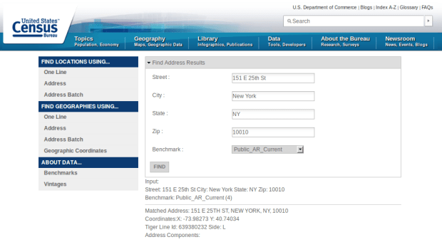
The Census Bureau’s TIGER and address files are often used as the foundational layers for building these other services, to which the service providers add refinements and improvements. You can access the Census Bureau’s services directly through the Census Geocoder, where you can match an address one at a time, or you can upload a batch of 1000 records. It returns longitude and latitude coordinates in NAD 83, and you can get names and codes for all the census geographies where the address is located. The service is pretty picky about the structure of the upload file (must be plain text, csv, with an id column and then columns with the address components in a specific order – with no other attributes allowed) but the nice thing is it requires no login and no key. It’s also public domain, so you can do whatever you want with the data you’ve retrieved. A tutorial for using it is available on our lab’s census tutorials page.

They also have an API with some basic documentation. You can match parsed and unparsed addresses, and can even do reverse geocoding. So I took a stab at writing a script to batch process addresses in text-delimited files (csv or txt). Unfortnately, the Census Geocoding API is not one of the services covered by the Python Geocoder that I mentioned in my previous post, but I did find another third party module called censusgeocode which provides a thin wrapper you can use. I incorporated that module into my Python 3 script, which I wrote as a function that takes the following inputs:
census_geocode(datafile,delim,header,start,addcol) (str,str,str,int,list[int]) -> files

datafile – this is the name of the file you want to process (file name and extension). If you place the geocode_census_funct.py file in the same directory as your data file, then you just need to provide the name of the file. Otherwise, you need to provide the full path to the file.
delim – this is the delimiter or character that separates the values in your data file. Common delimiters includes commas ‘,’, tabs ‘t’, and pipes ‘|’.
header – here you specify whether your file has a header row, i.e. column names. Enter ‘y’ or ‘yes’ if it does, ‘n’ or ‘no’ if it doesn’t.
start – type 0 to specify that you want to start reading the file from the beginning. If you were previously running the script and it broke and exited for some reason, it provides an index number where it stopped reading; if that’s the case you can provide that index number here, to pick up where you left off.
addcol – provide a list that indicates the position number of the columns that contain the address components in your data file. For an unparsed address, you provide just one position number. For a parsed address, you provide 4 positions: address, city, state, and ZIP code. Whether you provide 1 or 4, the numbers must be supplied in brackets, as the function requires a Python list.

You can open the script in IDLE, run it to load it into memory, and then type the function with the necessary parameters in the shell to execute it. Some examples:

A tab-delimited, unparsed address file with a header that’s stored in the same folder as the script. Start from the beginning and the address is in the 2nd column: census_geocode('my_addresses.txt','t','y',0,[2])
A comma-delimited, parsed address file with no header that’s stored in the same folder as the script. Start from the beginning and the addresses are in the 2nd through 5th columns: census_geocode('addresses_to_match.csv',',','n',0,[2,3,4,5])
A comma-delimited, unparsed address file with a header that’s not in the same folder as the script. We ran the file before and it stopped at index 250, so restart there – the address is in the 3rd column: census_geocode('C:address_datadata1.csv',',','y',250,[3])

The beginning of the script “sets the table”: we read the address columns into variables, create the output files (one for matches, one for non-matches, and a summary report), and we handle whether or not there’s a header row. For reading the file I used Python’s CSV module. Typically I don’t use this module, as I find it’s much simpler to do the basic: read a line in, split it on a delimiter, strip whitespace, read it into a list, etc. But in this case the CSV module allows you to handle a wider array of input files; if the input data was a csv and there happened to be commas embedded in the values themselves, the CSV module easily takes care of it; if you ignore it, the parsing would get thrown off for that record.

Handling Exceptions and Server Errors

In terms of expanding my skills, the new things I had to learn were exception handling and control flows. Since the censusgeocoding module is a thin wrapper, it had no built in mechanism for retrying a match a certain number of times if the server timed out. This is an absolute necessity, because the census server often times out, is busy, or just hiccups, returning a generic error message. I had already learned how to handle crashes in my earlier geocoding experiments, where I would write the script to match and write a record one by one as it went along. It would try to do a match, but if any error was raised, it would exit that loop cleanly, write a report, and all would be saved and you could pick up where you left off. But in this case, if that server non-response error was returned I didn’t want to give up – I wanted to keep trying.

So on the outside there is a loop to try and do a match, unless any error happens, then exit the loop cleanly and wrap up. But inside there is another try loop, where we try to do a match but if we get that specific server error, continue: go back to the top of that for loop and try again. That loop begins with While True – if we successfully get to the end, then we start with the next record. If we get that server error we stay in that While loop and keep trying until we get a match, or we run out of tries (5) and write as a non-match.

In doing an actual match, the script does a parsed or unparsed match based on user input. But there was another sticking point; in some instances the API would return a matched result (we got coordinates!), but some of the objects that it returned were actually errors because of some java problem (failed to get the tract number or county name – here’s an error message instead!) To handle this, we have a for i in range loop. If we have a matched record and we don’t have a status message (that indicates an error) then we move along and grab all the info we need – the coordinates, and all the census geography where that coordinate falls, and write it out, and then that for loop ends with a break. But if we receive an error message we continue – go back to the top of that loop and try doing the match again. After 3 tries we give up and write no match.

Figuring all that out took a while – where do these loops go and what goes in them, how do I make sure that I retry a record rather than passing over it to the next one, etc. Stack Exchange to the rescue! Difference between continue, pass and break, returning to the beginning of a loop, breaking out of a nested loop, and retrying after an exception. The rest is pretty straightforward. Once the matching is done we close the files, and write out a little report that tells us how many matches we got versus fails. The Census Geocoder via the API is pretty unforgiving; it either finds a match, or it doesn’t. There is no match score or partial matching, and it doesn’t give you a ZIP Code or municipal centroid if it can’t find the address. It’s all or nothing; if you have partial or messy addresses or PO Boxes, it’s pretty much guaranteed that you won’t get matches.

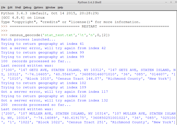
There’s no limit on number of matches, but I’ve built in a number of pauses so I’m not hammering the server too hard – one second after each match, 5 seconds after every 1000 matches, a couple seconds before retrying after an error. Your mileage will vary, but the other day I did about 2500 matches in just under 2 hours. Their server can be balky at times – in some cases I’ve encountered only a couple problems for every 100 records, but on other occasions there were hang-ups on every other record. For diagnostic purposes the script prints every 100th record to the screen, as well as any problems it encountered (see pic below). If you launch a process and notice the server is hanging on every other record and repeatedly failing to get matches, it’s probably best to bail out and come back later. Recently, I’ve noticed fewer problems during off-peak times: evenings and weekends.

script_running

Wrap Up

The script and the documentation are posted on our labs resources page, for all to see and use – you just have to install the third party censusgeocode module before using it. When would you want to use this? Well, if you need something that’s free, this is a good choice. If you have batches in the 10ks to do, this would be a good solution. If you’re in the 100ks, it could be a feasible solution – one of my colleagues has confirmed that he’s used the script to match about 40k addresses, so the service is up to the task for doing larger jobs.

If you have less than a couple thousand records, you might as well use their website and upload files directly. If you’re pushing a million or more – well, you’ll probably want to set up something locally. PostGIS has a TIGER module that lets you do desktop matching if you need to go into the millions, or you simply have a lot to do on a consistent basis. The excellent book PostGIS in Action has a chapter dedicated to to this.

In some cases, large cities or counties may offer their own geocoding services, and if you know you’re just going to be doing matches for your local area those sources will probably have greater accuracy, if they’re adding value with local knowledge. For example, my results with NYC’s geocoding API for addresses in the five boroughs are better than the Census Bureau’s and is customized for local quirks; for example, I can pass in a borough name instead of a postal city and ZIP Code, and it’s able to handle those funky addresses in Queens that have dashes and similar names for multiple streets (35th st, 35th ave, 35th dr…). But for a free, public domain service that requires no registration, no keys, covers the entire country, and is the foundation for just about every US geocoding platform out there, the Census Geocoder is hard to beat.

Python Geocoding Take 1 – International Addresses

This past semester has been the semester of geocoding. I’ve had a number of requests for processing large batches of addresses. Now that the term is drawing to a close, I’ll share some of my trials and tribulations. In this post, I’ll focus on my adventures in international geocoding.

First, it’s necessary to provide some context. As an academic librarian I’m primarily engaged with assisting students and faculty with their coursework and their research. My users are interested in getting coordinates for data so that they can do both analysis and visualization, which requires them to download the actual coordinate data in a batch and integrate it with the rest of their projects.

This is an important distinction to make, because in many cases the large web mapping companies (Google, Bing, Mapquest, etc) are not catering to this population – they provide services and APIs to web developers, so these folks can integrate geocoding services into the Google, Bing, etc maps they are embedding in their website. They geocoding providers specifically prohibit (in the fine print of their terms of use) anyone from using their services to create and download geocoded data. This essentially excludes a lot of academic use – which, is something I hadn’t fully grasped at the outset.

Google’s Geocoding API Perhaps?

My adventure began when a professor asked me for help in geocoding about 1 million addresses – in Turkey. Right from the beginning, many of the usual sources I would turn to (for US addresses) were out the window. I knew that I could do small scale batches of international addresses with the mmQGIS geocoding plugin, so I started testing there. The address file we had consisted of unparsed addresses, and the formating looked rather chaotic – but after doing some research I discovered that geocoding Turkish addresses was a tough proposition. The Open Street Map plugin (using Nominatim) returned no matches for our 1000 test cases. The Google results were much better, so we decided to investigate writing a script and using an API and to pay for the matching. According to the documentation, it would end up costing $500 to do 1 million addresses.

I searched around for some Python APIs and found what I believed was the official one for google maps geocoding. So I spent a day writing a script that would loop through the addresses, which we divided into batches of 100k records each (which is the max you can do per day with Google if you set up billing), and the professor obtained an API key and set up billing for the account. The interface for setting up and managing the Google APIs was ridiculously confusing. Eventually we were set and I let the script rip, and found that it wouldn’t rip for long. It would consistently stop after doing a few thousand records. I had written it to write results one by one as they were obtained, and to exit cleanly in the case of errors. Upon exit, it provides the index number of the record where it stopped, so I was able to pick up where it left off. But the server would constantly time out – sometimes it could do 10 to 12k records in a stretch, but often less, so I could never leave it unattended for long. The matches themselves were a mixed bag – you could throw absolute garbage at the Google geocoder and still get a match – if not to an address or property, then to a street segment, and beyond that to useless things like postal codes, administrative districts, and the country as a whole (i.e. I can’t find your address, so here are the coordinates for the geographic center of Istanbul, or for all of Turkey. Have a nice day).

It seemed like it was going to be a long climb to get to 1 million – but after about 100k we could go no further. Google simply refused every additional request. A new API key would get us a little further, but soon after that nothing would work and we wouldn’t get any useful error messages to explain why. Having never done anything like this before, I started to investigate why, and eventually discovered the problem: these web mapping geocoding services, even if you pay for them, are not meant to be used this way. Buried in the documentation I found the license restrictions, which stipulate that you are not allowed to download any of the data, and you had to plot every coordinate you retrieved onto a Google map. This is a service for web mapping developers, not researchers.

Why hadn’t I realized this before? One, I simply had never made this distinction as I thought geocoding was geocoding, and in my world of course people are going to want to download the coordinates. Two, the Internet is full of thousands of little blog posts and tutorials which demonstrate how to use the Google Maps APIs, so I thought this was possible. But they never mention any of the caveats about what you can and can’t do with these services. In addition to violating the service terms, what I was doing was akin to yelling in the back of a crowded room, as I was hammering their server, sending requests as fast as I could with no limit. A normal web mapping application (which is what the service is designed for) would send a fraction of those requests in that amount of time. No wonder the requests were refused. Thus ended my Google geocoding experiment.

Nope – How About ESRI Instead?

So what to do next? I found that most of the other commercial web mapping services didn’t provide anything near the maximum caps and low prices that Google was offering. Mapquest for example requires that you subscribe to an account on a monthly or annual basis, and 100k is the amount you could do in a month. Most of the other commercial services also prohibit any downloads.

The big exception is ESRI – they are one of the few that understand and cater to the academic market, and they do allow downloads: they say quite plainly: “Take your Coordinates with you. Once you have the results of a Geocode operation, they’re yours to take anywhere.” My university has a site license for ArcGIS, but it doesn’t include geocoding. You can create an account and have a certain number of free credits, and after that you pay. 1 mil records was going to cost about $4000 – substantially more than Google, but totally legal. ESRI provides lists of countries and ranks them according to how complete their street network coverage is. You can use their API via a script, or you can set up the service in ArcGIS Desktop and do the matching through the ArcToolbox. This would be painfully slow if you were doing a large job (like this one) but for the purpose of testing it out with a few hundred records this is what I tried. Unfortunately, in our case the results still weren’t good. Most of the addresses were to administrative or postal areas; not specific enough.

The Python Geocoder and a Wealth of Options

What often happens in librarianship when a patron makes an initial request (this should be a piece of cake, right?) and then discovers that what they’re looking for is more involved (ahhh this will be tougher than we thought), is that they reframe the question. He went back through the addresses with a research partner and winnowed them down based on what they really, absolutely needed, so now we were down from 1 million to just finding a match for about 300k. His colleague also suggested that we use Yandex, the Russian search and mapping engine. The structure of Russian addresses is quite similar to Turkish ones, and since Russia is closer to Turkey geographically and economically Yandex might do a better job.

I was dubious of this at first, but was quickly surprised. I found the Python Geocoder module, which provides a common, uniform API to over two dozen different geocoding services – including Google. Given the simplicity and flexibility of this module, it’s the one I should have used in the first place. And while Google limits you to 2500 free matches in one day, Yandex allows you 25k – that’s 25,000 – free matches in one day, without having to request an API key! I modified the original script I wrote to use the Python Geocoder module with Yandex, and the initial small-batch tests were successful. Here’s a small portion of the code – it loops through a file where the address is stored in one field (unparsed):

for index, line in enumerate(readfile):
        address=line.strip().split(delim)
        result=geocoder.yandex(address[add]).json

And it spits you back this JSON result (you could also do XML if you prefer):

{‘quality’: ‘street’, ‘address’: ‘Türkiye, İstanbul, Fatih, Cankurtaran Mh., Ayasofya Meydanı’, ‘location’: ‘Hagia Sophia Museum, Sultanahmet Mh., Ayasofya Meydanı, Fatih/İstanbul’, ‘state’: ‘İstanbul’, ‘lng’: ‘28.979031’, ‘accuracy’: ‘street’, ‘encoding’: ‘utf-8’, ‘provider’: ‘yandex’, ‘country_code’: ‘TR’, ‘ok’: True, ‘status_code’: 200, ‘lat’: ‘41.00772’, ‘country’: ‘Türkiye’, ‘county’: ‘Fatih’, ‘confidence’: 10, ‘bbox’: {‘northeast’: [41.008156, 28.979714], ‘southwest’: [41.007285, 28.978349]}, ‘street’: ‘Ayasofya Meydanı’, ‘status’: ‘OK’}

If the result you get back is not OK (ok is False – nothing matched), then write the record to the unmatched file. Otherwise, get the bits and pieces out of the json object that you want, append them to the record, and write the whole record out to a matched file.

        if result.get('ok')==False:
                nomatch.append(address)
                nomatchfile.writelines('t'.join(address)+'n')
        else:
                lng=result.get('lng')
                lat=result.get('lat')
                qual=result.get('quality')
                accu=result.get('accuracy')
                matchadd=result.get('address')
                newitems=lng,lat,qual,accu,matchadd
                address.extend(newitems)
                matched.append(address)
                matchfile.writelines('t'.join(address)+'n')

But is it legal? It was unclear to me; they specify that map data is meant for personal/noncommercial use and in the same sentence: “Any copying of the Data, their reproduction, conversion, distribution, promulgation (publication) in the Internet, any use of the Data in mass media and/or for commercial purposes without a prior written consent of the right holder, shall be prohibited”. Does that mean any copying, or just copying for commercial use or for redistributing the data? In our case, this is for academic non-profit use and the data (individual geocoded records) wasn’t going to be republished – it would be used for plotting distances between locations and making highly generalized static dot maps for an article. At this stage we seemed to be out of options – if you need to geocode a large batch of international addresses, AND you are willing to pay for it, where on Earth can you go?

Ultimately, I left it up to the professor to contact them or not, and we decided to roll the dice. For my part, I engineered the script to put a minimum load on their servers – essentially I could take 24 hours to do 25k records. I used the time and random modules in Python to build pauses in between records to slow things down. In sharp contrast to Google, the Yandex servers were amazingly reliable – they were able to do batches of 25k records every single time without timing out – not even once – and in less than a couple weeks we were finished. About 50% of the matches were good, and for the others he and a research assistant went back and cleaned up unmatched records, and I gave them the script so they could try again.

International Geocoding: The Take-Aways

If you need to geocode a large batch of foreign addresses for academic or research purposes, forget Google. Their service was less than stellar (to put it mildly) and anyway it’s a violation of their license agreement. And all those lousy little blog posts out there that show you how to use the Google Map APIs with Python and say “Gee isn’t this great!” are largely useless for practical purposes.
The Python Geocoder module is simple to use and let’s you write a single script to access a ton of different geocoding services, including Open Streetmap, Yandex, and ESRI. But you still need to review the terms of service for each one to see what’s allowed and what the daily limits are.
If you have funding for your research project, and ESRI geocoding has good coverage for your geographic area (based on their documentation but also on your own testing) then go with them, as you’re free and clear to download data under their terms. Arc Desktop will be too sluggish for large batches so write a script – you can use the Python Geocoder.
Otherwise – the Open Street Map / Nominatim services are worth a try but your success will vary by country. I had used them before for addresses in France with fair success, but it didn’t help me with Turkey.
You can also crawl through the GIS Stackexchange for advice. I’ve found that most of the suggestions are either for US geocoding, or are companies that are answering posts saying “Hey you can try my service!”

Happy geocoding, comrades! In my next post I’ll discuss my experience with batch geocoding addresses here in the US of A with Python.

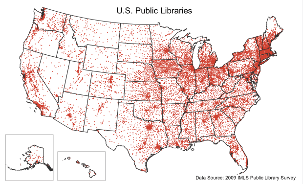
Average Distance to Public Libraries in the US

A few months ago I had a new article published in LISR, but given the absurd restrictions of academic journal publishing I’m not allowed to publicly post the article, and have to wait 12 months before sharing my post-print copy. It is available via your local library if they have a subscription to the Science Direct database (you can also email me to request a copy). .

Citation and Abstract

Regional variations in average distance to public libraries in the United States
F. Donnelly
Library & Information Science Research
Volume 37, Issue 4, October 2015, Pages 280–289
http://dx.doi.org/10.1016/j.lisr.2015.11.008

Abstract

“There are substantive regional variations in public library accessibility in the United States, which is a concern considering the civic and educational roles that libraries play in communities. Average population-weighted distances and the total population living within one mile segments of the nearest public library were calculated at a regional level for metropolitan and non-metropolitan areas, and at a state level. The findings demonstrate significant regional variations in accessibility that have been persistent over time and cannot be explained by simple population distribution measures alone. Distances to the nearest public library are higher in the South compared to other regions, with statistically significant clusters of states with lower accessibility than average. The national average population-weighted distance to the nearest public library is 2.1 miles. While this supports the use of a two-mile buffer employed in many LIS studies to measure library service areas, the degree of variation that exists between regions and states suggests that local measures should be applied to local areas.”

Purpose

I’m not going to repeat all the findings, but will provide some context.

As a follow-up to my earlier work, I was interested in trying an alternate approach for measuring public library spatial equity. I previously used the standard container approach – draw a buffer at some fixed distance around a library and count whether people are in or out, and as an approximation for individuals I used population centroids for census tracts. In my second approach, I used straight-line distance measurements from census block groups (smaller than tracts) to the nearest public library so I could compare average distances for regions and states; I also summed populations for these areas by calculating the percentage of people that lived within one-mile rings of the nearest library. I weighted the distances by population, to account for the fact that census areas vary in population size (tracts and block groups are designed to fall within an ideal population range – for block groups it’s between 600 and 3000 people).

Despite the difference in approach, the outcome was similar. Using the earlier approach (census tract centroids that fell within a library buffer that varied from 1 to 3 miles based on urban or rural setting), two-thirds of Americans fell within a “library service area”, which means that they lived within a reasonable distance to a library based on standard practices in LIS research. Using the latest approach (using block group centroids and measuring the distance to the nearest library) two-thirds of Americans lived within two miles of a public library – the average population weighted distance was 2.1 miles. Both studies illustrate that there is a great deal of variation by geographic region – people in the South consistently lived further away from public libraries compared to the national average, while people in the Northeast lived closer. Spatial Autocorrelation (LISA) revealed a cluster of states in the South with high distances and a cluster in the Northeast with low distances.

The idea in doing this research was not to model actual travel behavior to measure accessibility. People in rural areas may be accustomed to traveling greater distances, public transportation can be a factor, people may not visit the library that’s close to their home for several reasons, measuring distance along a network is more precise than Euclidean distance, etc. The point is that libraries are a public good that provide tangible benefits to communities. People that live in close proximity to a public library are more likely to reap the benefits that it provides relative to those living further away. Communities that have libraries will benefit more than communities that don’t. The distance measurements serve as a basic metric for evaluating spatial equity. So, if someone lives more than six miles away from a library that does not mean that they don’t have access; it does means they are less likely to utilize it or realize it’s benefits compared to someone who lives a mile or two away.

Data

I used the 2010 Census at the block group level, and obtained the location of public libraries from the 2010 IMLS. I improved the latter by geocoding libraries that did not have address-level coordinates, so that I had street matches for 95% of the 16,720 libraries in the dataset. The tables that I’m providing here were not published in the original article, but were tacked on as supplementary material in appendices. I wanted to share them so others could incorporate them into local studies. In most LIS research the prevailing approach for measuring library service areas is to use a buffer of 1 to 2 miles for all locations. Given the variation between states, if you wanted to use the state-average for library planning in your own state you can consider using these figures.

To provide some context, the image below shows public libraries (red stars) in relation to census block group centroids (white circles) for northern Delaware (primarily suburban) and surrounding areas (mix of suburban and rural). The line drawn between the Swedesboro and Woodstown libraries in New Jersey is 5-miles in length. I used QGIS and Spatialite for most of the work, along with Python for processing the data and Geoda for the spatial autocorrelation.

The three tables I’m posting here are for states: one counts the 2010 Census population within one to six mile rings of the nearest public library, the second is the percentage of the total state population that falls within that ring, and the third is a summary table that calculates the mean and population-weighted distance to the nearest library by state. One set of tables is formatted text (for printing or just looking up numbers) while the other set are CSV files that you can use in a spreadsheet. I’ve included a metadata record with some methodological info, but you can read the full details in the article.

All tables in TXT and CSV format

In the article itself I tabulated and examined data at a broader, regional level (Northeast, Midwest, South, and West), and also broke it down into metropolitan and non-metropolitan areas for the regions. Naturally people that live in non-metropolitan areas lived further away, but the same regional patterns existed: more people in the South in both metro and non-metro areas lived further away compared to their counterparts in other parts of the country. This weekend I stumbled across this article in the Washington Post about troubles in the Deep South, and was struck by how these maps mirrored the low library accessibility maps in my past two articles.

Review of The Census Reporter

Picking up where I left off from my previous post (gee – welcome to 2016!) I thought I’d give a brief review of another census resource, The Census Reporter at http://censusreporter.org/.

The Census Reporter was created to make it easier for journalists to write stories using census data. To that end, they’ve created a really slick and easy to use web site that makes the data accessible and fun to explore. From the homepage you have three ways of diving into the data: you can pull up a profile by typing in the name of a place, you can enter an address and explore places that contain that address, or you can explore tables by topic.

First, the place-based approach. You can type in a named place, like a state, county, or a census place (incorporated cities and towns, or census designated places) to get started. This will give you a selection of data from the most recent release of the American Community Survey. For larger areas where the data is available, it gives you 1-year ACS data by default; otherwise you get the latest 5-year data.

You’re presented with a map of the location at the top, and a series of attractive looking graphs and charts sorted by the demographic profile table source – social, economic, housing, and demographic. If you hover over a data point in a table it gives you some geographic context by comparing this place’s value with that of larger places where it’s contained. For example, if I search for Philadelphia I can hover over the chart to get the value for the Philly metro area and the State of Pennsylvania. I can click a link below each chart to open the full table, which includes both estimates and margins of error. There are small links for viewing the table by itself on a separate page (which also gives you the ability to download it) and for embedding the chart in a website.

Viewing the table gives you additional options, like adding additional places for comparison, or subdividing the place into smaller areas for comparison. So if I’m looking at Philadelphia, I can break it down into tracts, block groups, or ZIP Codes. From there I can toggle away from the table view to view a map or a distribution bar to explore that variable by individual geographies.

The place-based search is great at allowing you to drill down either by topic or by these smaller geographies. But if you wanted to access a fuller range of geographies like congressional districts or PUMAs, it seems easier to do an address-based search. Back on the homepage, selecting the address button and typing in an address brings you to a map with the address pin-pointed, and on the left you can choose any geography that encloses that address. Once you do that, you get a profile for that geography and can start doing the same sorts of operations for changing the topics or tables, or adding or subdividing geographies for comparison.

The topic-based search lets you search just by topic and then figure out the geography piece later. Of the three types of searches this one is the toughest, given the sheer number of tables and cross-tabulations. You can click on a link for a general topic to narrow things down a bit before beginning a search.

In downloading the data you have a variety of useful options: CSV, Excel, GeoJSON, KML, and shapefiles. So in theory you can download data that’s readily mappable – in practice I wasn’t able to download a shapefile, but could grab a KML or GeoJson and was able to visualize it in QGIS. One challenge in downloading any of the files is that the column names use the identifier codes, and the actual names of the variables aren’t included in the download format you choose – they’re included in a json file. So you can use that for reference, but it can’t be readily incorporated into the table.

So – where would this resource fall within the pantheon of US Census data resources? I think it’s great for accessing and, especially, visualizing profiles (profile = lots of data for one place) from the most recent ACS releases. It’s easy to use and succeeds at making the data interesting; for that reason I certainly would incorporate it into undergraduate courses where I’m introducing data. The ability to embed the charts into websites is certainly a bonus, and they deserve a big thumbs up for incorporating the margin of error data, rather than hiding or discarding it like other resources do.

The ability to create and view comparison tables (comparison = one piece of data for many places) is good – select an area and then break it down – but not as strong as the profile options. If you want to get a profile for a non-named place like a tract, ZIP Code, or PUMA you can’t do that from the profile search. You can do an address search and back out (if you know an address for that you’re interested in) or you can drill down by topic, which lets you search by summary area in addition to named places.

For users who need to download a lot of data, or for folks who need datasets that aren’t the most recent ACS release, this resource isn’t the place to go. The focus here is on providing the data in an easy and compelling way, as is. In viewing the profiles, it’s not clear if you can choose 5-year data over 1-year data for places where both datasets are available – even for large geographic areas with high population, sometimes it’s preferable to use the 5-year data to take advantage of the smaller margins of error. I also didn’t see an option for choosing decennial census data.

In short, this resource is well-designed and definitely worth exploring. It seems clear why this would be a go-to source for journalists, but it can be for many others as well.