latex

Recent Migration Trends for New York City and Metro

The Baruch GIS lab crew just published a paper: New Yorkers on the Move: Recent Migration Trends for the City and Metro Area. The paper (no. 15 Feb 2018) is part of the Weissman Center for International Business Occasional Paper Series, which focuses on New York City’s role in the international and domestic economy.

Findings

We analyzed recent population trends (2010 to 2016) in New York City and the greater metropolitan area using the US Census Bureau’s Population Estimates to study components of population change (births, deaths, domestic and international migration) and the IRS Statistics of Income division’s county to county migration data to study domestic migration flows.

Here are the main findings:

The population of New York City and the New York Metropolitan Area increased significantly between 2010 and 2016, but annually growth has slowed due to greater domestic out-migration.
Compared to other large US cities and metro areas, New York’s population growth depends heavily on foreign immigration and natural increase (the difference between births and deaths) to offset losses from domestic out-migration.
Between 2011 and 2015 the city had few relationships where it was a net receiver of migrants (receiving more migrants than it sends) from other large counties. The New York metro area had no net-receiver relationships with any major metropolitan area.
The city was a net sender (sending more migrants than it received) to all of its surrounding suburban counties and to a number of large urban counties across the US. The metro area was a net sender to metropolitan areas throughout the country.

For the domestic migration portion of the analysis we were interested in seeing the net flows between places. For example, the NYC metro area sends migrants to and receives migrants from the Miami metro. What is the net balance between the two – who receives more versus who sends more?

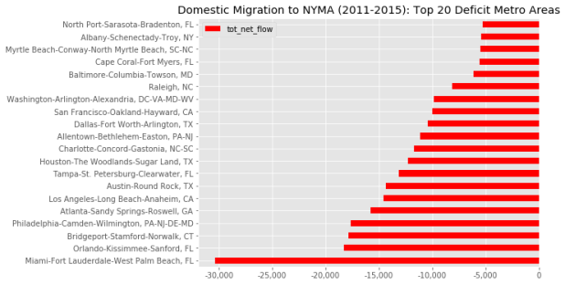
The answer is: the NYC metro is a net sender to most of the major metropolitan areas in the country, and has no significant net receiver relationships with any other major metropolitan area. For example, for the period from 2011 to 2015 the NYC metro’s largest net sender relationship was with the Miami metro. About 88,000 people left the NYC metro for metro Miami while 58,000 people moved in the opposite direction, resulting in a net gain of 30,000 people for Miami (or in other words, a net loss of 30k people for NYC). The chart below shows the top twenty metros where the NYC metro had a deficit in migration (sending more migrants to these areas than it received). A map of net out-migration from the NYC metro to other metros appears at the top of this post. In contrast, NYC’s largest net receiver relationship (where the NYC metro received more migrants than it sent) was with Ithaca, New York, which lost a mere 300 people to the NYC metro.

All of our summary data is available here.

Process

For the IRS data we used the county to county migration SQLite database that Janine meticulously constructed over the course of the last year, which is freely available on the Baruch Geoportal. Anastasia employed her Python and Pandas wizardry to create Jupyter notebooks that we used for doing our analysis and generating our charts, all of which are available on github. I used an alternate approach with Python and the SQLite and prettytable modules to generate estimates independently of Anastasia, so we could compare the two and verify our numbers (we were aggregating migration flows across years and geographies from several tables, and calculating net flows between places).

One of our goals for this project was to use modern tools and avoid the clunky use of email. With the Jupyter notebooks, git and github for storing and syncing our work, and ShareLaTeX for writing the paper, we avoided using email for constantly exchanging revised versions of scripts and papers. Ultimately I had to use latex2rtf to convert the paper to a word processing format that the publisher could use. This post helped me figure out which bibliography packages to choose (in order for latex2rtf to interpret citations and references, you need to use the older natbib & bibtex combo and not biblatex & biber).

If you are doing similar research, Zillow has an excellent post that dicusses the merits of the different datasets. There are also good case studies on Washington DC and Philadelphia that employ the same datasets.

Note Taking for Academic Research

I’ve been reviewing a lot of literature over the past year in preparation for writing my book, so note taking is at the forefront of my mind. Grad students occasionally ask me for suggestions on how to effectively take notes, so I’ll share some pointers here. I’ll begin with my quest to find the right note taking software, followed by my actual process for taking notes.

Finding the Right Tool

Ten years ago, I suddenly found myself back in a position where I needed to write academic papers, something I hadn’t done since I wrote my master’s thesis about eight years before that. At that time, I was still using the techniques I had learned in high school (a much longer time ago…). Back then, you were either an index card person or a binder person. The card people would write one note on each card, while binder people kept a ledger of notes and would add additional pages as needed. You’d classify your notes as summaries, paraphrases, or quotations.

I assumed that my high school methods must be outdated by now, so I cast around to see what note taking software was available. I knew I wanted to go open source, as I didn’t want my notes tethered to a specific tool and stored in proprietary format. There were a lot of options, and I quickly became bogged down and frustrated with trying them all. I felt that much of the software forced me to conform to it, and I was spending too much time fidgeting and figuring things out.

I abandoned the search and recorded my notes in a simple text (aka notepad) document. I had always been a binder person, so the single document approach appealed to me. I could copy and paste, use spell check, and search for keyword terms that I assigned (the Linux editors like gedit, leafpad, and xed are lightweight but more robust than MS Notepad). This worked fine for a stand-alone paper and I still use this approach for small projects. But as my research became on-going I needed to rely on these notes for many future projects. The single notepad document grew unwieldy and browsing and searching became difficult.

A few years later, I made a second attempt at searching for note taking software, and this time I broadened the search to include more general-purpose options. My solution: use a wiki! With a wiki, every single source can have it’s own page, the sources can be grouped together under thematic categories, you can assign tags, and you can search across all the pages. I could also add links between pages and out to the web, and could link the notes to the source documents. The wiki was so open ended that I didn’t feel constrained in writing my notes to fit a particular interface, nor did I have to waste a lot of time sifting though buttons and tools.

I opted for a desktop wiki called Zim, which has been actively maintained since 2008. All of the pages in Zim are saved as individual text files in a basic wiki mark-up, which insures that they can be accessed outside the program. Pages are stored in a notebook which is essentially just a folder. If you create hierarchies of pages, these categories become folders and sub-folders. Zim has a ton of extra plugins so you can do spell checking, concept mapping, you can create formulas, calendars, and more. You can also export your entire notebook or portions of it out as HTML or LaTeX files.

Most importantly, the wiki solved one of my most vexing problems. I found that a lot of the note taking software was geared towards just taking notes, and couldn’t handle keeping track of citations. Citation software is it’s own genre, and I found that those packages were poor for taking notes. With Zim, I create a page dedicated to each source, and at the top of each page I embed some BibTeX code for storing the citation data. BibTeX is a format that’s used for creating LaTeX bibliographies, but it has become a common standard and can be used by word processors too. I have a template page (see below) with several BibTeX document types that I just copy and paste when I have a new source to add. Since the pages are saved as plain text, I wrote a short Python script (appears at the end of this post) that loops through my note pages, scrapes out the BibTeX records, and creates a BibTeX file that I can use in LaTeX. Within the BibTeX record I store a link to the source: either to a PDF I have locally, or a web page (if it’s a site), or a WorldCat catalog record (if it’s a book). So all my notes, citations, and the source material are kept together in one place!

BibTeX templates

Zim is desktop software that you have to download and install locally. Since the notebook consists of text files in folders, it’s easy to back it up into Box or DropBox or whatever you use. Zim doesn’t save histories or have version control, but there’s a plugin that lets you sync your files with Git and other systems.

Relying on Tried and True Methods

While the right tool is important, it’s really the method that counts. I learned that I had to jettison the idea that the note taking process has to be 100% efficient. While you certainly don’t want to flail around and waste time, note taking is not supposed to be quick and easy. The only way you can truly learn new material is to spend time with it: reading, re-reading, taking notes, and reading the notes. The process of note taking is equally if not more important than the actual notes themselves, as the process is what helps you to synthesize and learn the material. While I left the binder and note cards behind, the actual note taking process was similar to what I did in high school.

I always download articles and bookmark websites or catalog records as I’m doing my searches. Once I complete a series of searches and have gathered material from the web and library databases, I sift through the files and rename them using the first author’s last name and the year of publication (i.e. Jones2017). I’ll also use this file name as the BibTeX key that uniquely identifies the article. I create a documents folder with sub-folders for articles, books, and reports, and I keep these folders in the same location as the ZIM notebook. There’s no reason to create lots of topical or thematic folders, as you can use the wiki to categorize and tag the notes, and the wiki becomes the vehicle for searching or browsing through the documents.

As I sort through the sources I identify what’s essential and what’s ancillary. High priority sources will be read thoroughly and covered in detail, while the low-priority stuff will be skimmed and summarized. High priority sources are critical to your research and include touchstone articles in your field, excellent case studies, relevant background material, and any past research that remotely resembles what you’re working on. Low priority sources may have one important fact or concept that you need to remember; these materials are more tangential to your work and ultimately you might cite them in passing, or even not at all.

I always print out the high-priority articles. I’ll read it first, and then I’ll go back and do a second read and mark passages with a high-lighter. Next, I’ll create and type notes directly into the wiki. I might read and mark up a couple articles before I start note taking, but I don’t wait too long as I want the articles fresh in my memory. For essential books, I’ll read a chapter or two at a time and mark passages with little sticky flags. Then I’ll go back and take notes in a paper notebook, and will keep doing that until I finish the book. Then I transcribe all the notes for the book onto my laptop. This takes longer, but once again it’s not all about efficiency. I get to spend more time with the material and it helps me absorb it. This approach also separates the computer from the reading, which cuts down distractions and provides more flexibility in terms of where I can work. Reading in a comfortable chair or outside is preferable to reading while sitting at a table with a laptop.

Note flags in book

I never print out or mark up low-priority articles; I skim through the digital copies and write a summary directly in the wiki. For books, I read the book in one go and may use sticky flags here and there, and when I’m done I type the notes directly into the wiki.

For the notes themselves, each note page has the title and author prominently at the top followed by a summary of the source, and then the BibTeX citation (see below). Low-priority materials usually get nothing but a summary and a citation. High-priority materials get detailed notes. Each note is written as a bullet point, and can represent one important fact or insight, or can be a summary of a paragraph or several pages, or even a summary of a chapter. It depends on how important the material is relative to my work.

Zim Wiki

Taking notes is not like writing a book report. I’m not writing an even or objective summary of the material in it’s entirety. Instead, I’m picking out the pieces that are of interest to me and to the work I’ll be doing, and I skip the rest. Sometimes I’ll editorialize (this is great, or this stinks) but I write in such a way that my thoughts are distinct from what the author is saying. This is where efficiency comes into the picture: identify sources that are high versus low priority, and summarize the source and identify just the specific details that are relevant to you. You’re writing these notes with specific research goals in mind, so don’t waste time writing a generic book report.

I always summarize or paraphrase the material as I take notes, putting concepts in my own words. Doing this forces you to wrestle with the concepts and internalize them, which improves your understanding of the material and your memory for it. It also helps guard against plagiarism; once you start writing the paper, you’ll know your notes are already in your own words and you can use them freely. If I do quote something directly, I always surround it with quotation marks. Lastly, at the end of my note I provide the page numbers to indicate what’s been summarized, so I can go back if need be.

Note taking is an idiosyncratic process. What works for you may not work for someone else and vice versa. The key is to figure out what works best for you; create a system, try it out, and once you’re happy go with it. You can always tweak things as you move along. The notes will help you when it comes time to pull your ideas together into a cohesive paper, but it’s the reading and note taking process that helps you to become proficient with the subject matter.

As I was re-learning how to take notes, I found the handouts from the University of Melbourne’s Academic Skills Unit to be particularly valuable. This is their latest version of Taking Notes From Texts, and this is the older version that I stumbled on years ago.

(Python code for scraping BibTeX records out of wiki notes to create a bibliography is posted below).

#Parse notes stored in zim wiki to extract all bibtex records and write them
#to a new bibtex file named with today's date.

#Script must be stored directly above the notes folder where the wiki data
#is stored. It will ignore the empty bibtex template files and will only
#read wiki files stored as .txt.

#Within the wiki, all bibtex records in the notes are enclosed in a bibtex tag.
#The script reads each line and ignores them until it finds the open
#tag. Then it starts writing each line until it reads the close  tag.
#A line return is appended so records are separated in the output file.

#A list and count of extracted records is provided as a diagnostic

import os, datetime

now=datetime.date.today()
path='.'
outfile='sources_'+str(now)+'.bib'

writefile=open(outfile,'w')

counter=0
titles=[]

for (subdir,dirs,files) in os.walk(path):
    if 'Templates' in dirs:
        dirs.remove('Templates')
    if 'documents' in dirs:
        dirs.remove('documents')
    for f in files:
        if f[-4:]=='.txt':
            readfile=open(os.path.join(subdir,f),'r')
            for line in readfile:
                if line.startswith('&lt;bibtex&gt;'):
                    break
            for line in readfile:
                if line.startswith('&lt;/bibtex'):
                    titles.append(f)
                    writefile.write('\n')
                    counter=counter+1
                    break
                else:
                    writefile.write(line)
            readfile.close()
writefile.close()

titles = [t.replace('_', ' ') for t in titles]
titles=[t.strip('.txt') for t in titles]
titles.sort()
print('Bibliographic records have been extracted for the following sources:','\n')
for title in titles:
    print('*',title)
print('\n')
print(counter,'bibilographic records have been parsed and written to',outfile)

Writing Functions and Building a Jinja Template

In previous posts I demonstrated how to pull data from a sqlite / spatialite data to generate reports using Python and Jinja, where Jinja2 is used as a template engine for creating LaTeX documents and the NYC Geodatabase is used as my test case. Up until now the scripts pulled the data “as is”. In this post I’ll demonstrate how I created derived variables, and how I created the Jinja2 template for the report. Please note – instead of duplicating all of the code I’m just going to illustrate the new pieces – you should check out the earlier posts to see how all the pieces fit together.

Aggregating Variables

Aggregating census data is a pretty common operation, and when working with American Community Survey estimates it’s also necessary to calculate a new margin of error for each derived value. I wrote two functions to accomplish this. For each function you pass in the keys for values you want to aggregate, a name which will be the name of the new variable, and a dictionary that contains all the keys and values that were taken from a database table for a specific geography.

#Functions for summing individual values and calculating margins of error
#for individual values

def calc_sums(keys,name,adict):
    tosum=[]
    for val in keys:
        tosum.append(adict.get(val))
    agg=sum(tosum)
    adict[name]=agg

def calc_moe(keys,name,adict):
    sqrd=[]
    for val in keys:
        item=adict.get(val)
        if item=='':
            pass
        else:
            sqrd.append(item**2)
    moe=round(math.sqrt(sum(sqrd)))
    adict[name]=moe

Later in the script, as we’re looping through all the geographies and gathering the necessary data into dictionaries that represent each data table, we call the function. In this example we’re combining household income brackets so that we don’t have so many categories:

for geog in geodict.keys():

    name=geodict.get(geog)
    filename='zzpuma_' + geog + '.tex'
    folder='puma_rept'
    outpath=os.path.join(folder,filename)

    acs1dict=pulltab('b_pumas_2013acs1','GEOID2',geog)
    acs2dict=pulltab('b_pumas_2013acs2','GEOID2',geog)

    calc_sums(['INC03_E','INC04_E'],'INC10K_E',acs1dict)
    calc_moe(['INC03_M','INC04_M'],'INC10K_M',acs1dict)
    calc_sums(['INC05_E','INC06_E'],'INC25K_E',acs1dict)
    calc_moe(['INC05_M','INC06_M'],'INC25K_M',acs1dict)
    calc_sums(['INC09_E','INC10_E'],'INC100K_E',acs1dict)
    calc_moe(['INC09_M','INC10_M'],'INC100K_M',acs1dict)

Rather than creating a new dictionary, these new values are simply appended to the existing dictionaries that contain the data taken from each of the ACS data tables in the database. They can be referenced in the template using their new column name.

Calculating Areas

I also want to include the geographic size of the PUMA as one of the report items. Columns for the area are included in the spatial table for the PUMAs – the features originally came from the TIGER files, and all TIGER files have an ALAND and an AWATER column that has land and water area in square meters. So we don’t have to calculate the area from the geometry – we can just use this function to convert the land and water attributes to square miles, and then calculate a total area:

def calc_area(adict,land,water,total):
    landarea=round(adict.get('aland10')*0.000000386102,2)
    waterarea=round(adict.get('awater10')*0.000000386102,2)
    totalarea=landarea+waterarea
    adict[land]=landarea
    adict[water]=waterarea
    adict[total]=totalarea

In the body of our script, we invoke our pulltab function (explained in an earlier post) to grab all the data from the PUMA spatial boundary table:

area=pulltab('c_bndy_pumas2010','geoid10',geog)

And then we can call our area function. We pass in the area dictionary, and what we want the new output column names to be – area for land, water, and total:

calc_area(area, 'LAND_SQM','WAT_SQM','TOT_SQM')

Like our previous aggregate script, this function appends our new values to the existing table-dictionary – in this case, one called area.

Aggregating Geographies

Our last function is a little more complicated. In all of our previous examples, we pulled PUMA-level data from the American Community Survey tables. What if we wanted 2010 Census data for the PUMAs? Decennial census data is not tabulated at the PUMA level, but it is tabulated at the census tract level. Since PUMAs are created by aggregating tracts, we can aggregate the census tract data in the NYC Geodatabase into PUMAs. Here’s our function:

#Function aggregates all values in a table with a group by field from a
#joined table, then creates a dictionary consisting of column names and values
#for a specific geography

def sumtab(tabname,jointab,id1,id2,gid,geog):
    query='SELECT * FROM %s LIMIT 1' %(tabname)
    curs.execute(query)
    col_names = [cn[0] for cn in curs.description]
    tosum=[]
    for var in col_names[3:]:
        tosum.append("SUM("+var+") AS '0_"+var+"'")
    summer=', '.join(str(command) for command in tosum)
    query='SELECT %s, %s FROM %s, %s WHERE %s = %s and %s = %s GROUP BY %s' %(gid,summer,tabname,jointab,id1,id2,gid,geog,gid)
    curs.execute(query)
    col_names = [cn[0] for cn in curs.description]
    rows = curs.fetchall()
    for row in rows:
        thedict=dict(zip(col_names,row))
    return thedict

What’s going on here? The first thing we need to do is associate the census tracts with the PUMAs they’re located in. The NYC Geodatabase does NOT have a relationship table for this, so I had to create one. We have to pass in the table name, the relationship table, the unique IDs for each, and then the ID and the geography that we’re interested in (remember our script is looping through PUMA geographies one by one). The first thing we do is a little trick – we get the names of every column in the existing data table, and we append them to a list where we create a new column name based on the existing one (in this case, append a 0 in front of the column name – in retrospect I realize this is a bad idea as column names should not begin with numbers, so this is something I will change). Then we can take the list of column names and create a giant string out of them.

With that giant string (called summer) we can now pass all of the parameters that we need into the SQL query. This selects all of our columns (using the summer string), the table names and join info, for the specific geographic area that we want and then groups the data by that geography (i.e. all tracts that have the same PUMA number). Then we zip the column names and values together in a dictionary that the function returns.

Later on in our script, we call the function:

   census10=sumtab('b_tracts_2010census','b_tracts_to_pumas','GEOID2','tractid','pumaid',geog)

Which creates a new dictionary called census10 that has all the 2010 census data for our PUMA. Like the rest of our dictionaries, census10 is passed out to the Jinja2 template and its values can be invoked using the dictionary keys (the column headings):

outfile=open(outpath,'w')
    outfile.write(template.render(geoid=geog, geoname=name, acs1=acs1dict, acs2=acs2dict, area=area,
                                  c2010=census10))
    outfile.close()

Designing the Template

The Jinja template is going to look pretty busy compared to our earlier examples, and in both cases they’re not complete (this is still a work in progress).

I wanted to design the entire report first, to get a sense for how to balance everything I want on the page, without including any Jinja code to reference specific variables in the database. So I initially worked just in LaTeX and focused on designing the document with placeholders. Ultimately I decided to use the LaTeX minipage environment as it seemed the best approach in giving me control in balancing items on the page. The LaTeX wikibook entries on floats, figures, and captions and on boxes was invaluable for figuring this out. I used rule to draw boxes to serve as placeholders for charts and figures. Since the report is being designed as a document (ANSI A 8 1/2 by 11 inches) I had no hang-up with specifying precise dimensions (i.e. this isn’t going into a webpage that could be stretched or mushed on any number of screens). I loaded the xcolor package so I could modify the row colors of the tables, as well as a number of other packages that make it easy to balance table and figure captions on the page (caption, subscaption, and multicol).

Once I was satisfied with the look and feel, I made a copy of this template and started modifying the copy with the Jinja references. The references look awfully busy, but this is the same thing I’ve illustrated in earlier posts. We’re just getting the values from the dictionaries we created by invoking their keys, regardless of whether we’re taking new derived values that we created or simply pulling existing values that were in the original data tables. Here’s a snippet of the LaTeX with Jinja that includes both derived (2010 Census, area) and existing (ACS) variables:

%Orientation - detail map and basic background info
begin{minipage}{textwidth}
	begin{minipage}[h]{3in}
   		centering
   		rule{3in}{3in}
    		captionof{figure}{Race by 2010 Census Tract}
	end{minipage}
  	hfill
	begin{minipage}[h]{4in}
		centering
		captionof{table}{Geography}
    	begin{tabular}{cccc}hline
		& Land & Water & Total\ hline
		Area (sq miles) &  num{VAR{area.get('LAND_SQM')}} & num {VAR{area.get('WAT_SQM')}} &  num {VAR{area.get('TOT_SQM')}} \ hline
		vspace{10pt}
	 end{tabular}
	captionof{table}{Basic Demographics}
	rowcolors{3}{SpringGreen}{white}
	 begin{tabular}{cccc}hline
		& textbf{2010 Census} & textbf{2009-2013} & textbf{ACS Margin}\
		& & textbf{ACS} & textbf{of Error}\ hline
		Population & num {VAR{c2010.get('0_HD01_S001')}} & num{VAR{acs2.get('SXAG01_E')}} & +/- num{VAR{acs2.get('SXAG01_M')}}\
		Males & num {VAR{c2010.get('0_HD01_S026')}} & num{VAR{acs2.get('SXAG02_E')}} & +/- num{VAR{acs2.get('SXAG02_M')}}\
		Females & num {VAR{c2010.get('0_HD01_S051')}}& num{VAR{acs2.get('SXAG03_E')}} & +/- num{VAR{acs2.get('SXAG03_M')}}\
		Median Age (yrs) & num {99999} & num{VAR{acs2.get('SXAG17_E')}} & +/- num{VAR{acs2.get('SXAG17_M')}}\
		Households & num {VAR{c2010.get('0_HD01_S150')}} & num{VAR{acs1.get('HSHD01_E')}} & +/- num{VAR{acs1.get('HSHD01_M')}}\
		Housing Units & num {VAR{c2010.get('0_HD01_S169')}} & num{VAR{acs2.get('HOC01_E')}} & +/- num{VAR{acs2.get('HOC01_M')}}\ hline
	end{tabular}
	end{minipage}
 end{minipage}

And here’s a snippet of the resulting PDF:

What Next?

You may have noticed references to figures and charts in some of the code above. I’ll discuss my trials and tribulations with trying to use matplotlib to create charts in some future post. Ultimately I decided not to take that approach, and was experimenting with using various LaTeX packages to produce charts instead.

Looping Through a Database to Create Reports

I’ve got a lot of ground to cover, picking up where I left off several months ago. In earlier posts I presented the concept for creating reports from sqlite databases using Python, Jinja, and LaTeX, and looked at different methods for passing data from the database to the template. I’m using the NYC Geodatabase as our test case. In this entry I’ll cover how I implemented my preferred approach – creating Python dictionaries to pass to the Jinja template.

One of the primary decisions I had to make was how to loop through the database. Since the reports we’re making are profiles (lots of different data for one geographic area), we’re going to want to loop through the database by geography. So, for each geography select all the data from a specific table, pass the data out to the template where the pertinent variables are pulled, build the report and move on to the next geography. In contrast, if we were building comparison tables (one specific variable for many geographic areas) we would want to loop through the data by variable.

In the beginning of the script we import the necessary modules, set up the Jinja environment, and specify our template (not going to repeat that code here – see the previous post). Then we have our function that creates a dictionary for a specific data table for a specific geography:

def pulltab(tabname,idcol,geog):
    query='SELECT * FROM %s WHERE %s = %s' %(tabname,idcol,geog)
    curs.execute(query)
    col_names = [cn[0] for cn in curs.description]
    rows = curs.fetchall()
    for row in rows:
        thedict=dict(zip(col_names,row))
    return thedict

We connect to the database and create a dictionary of all the geographies (limited to 3 PUMAs since this is just a test):

#Connect to database and create dictionary of all geographies

conn = sqlite3.connect('nyc_gdb_jan2015a/nyc_gdb_jan2015.sqlite')
curs = conn.cursor()
curs.execute('SELECT geoid10, namelsad10 FROM a_pumas2010 ORDER BY geoid10 LIMIT 3')
rows = curs.fetchall()
geodict=dict(rows)

And then we generate reports by looping through all the geographies in that dictionary, and we pass in the ID of each geography to pull all data from a data table for that geography out of the table and into a dictionary.

#Generate reports by looping through geographies and passing out
#dictionaries of values

for geog in geodict.keys():
    acs1dict=pulltab('b_pumas_2013acs1','GEOID2',geog)
    acs2dict=pulltab('b_pumas_2013acs2','GEOID2',geog)
    name=geodict.get(geog)
    filename='zzpuma_' + geog + '.tex'
    folder='test5'
    outpath=os.path.join(folder,filename)

Lastly, we pass the dictionaries out to the template, and run LaTeX to generate the report from the template:

  outfile=open(outpath,'w')
    outfile.write(template.render(geoid=geog, geoname=name, acs1=acs1dict, acs2=acs2dict))
    outfile.close()

    os.system("pdflatex -output-directory=" + folder + " " + outpath)

conn.close()

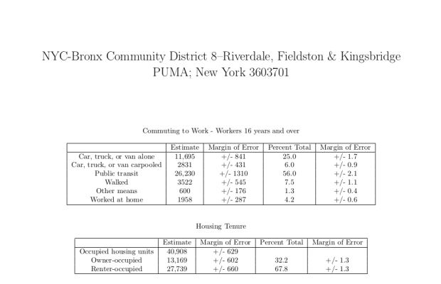
The Jinja template (as a LaTeX file) is below – the example here is similar to what I covered in my previous post. We passed two dictionaries into the template, one for each data table. The key is the name of the variable (the column name in the table) and the value is the American Community Survey estimate and the margin of error. We pass in the key and get the value in return. The PDF output follows.

documentclass{article}
usepackage[margin=0.5in]{geometry}
usepackage{graphicx}
usepackage[labelformat=empty]{caption}
usepackage[group-separator={,}]{siunitx}

title{VAR{acs1.get('GEOLABEL') | replace("&","&")} VAR{acs1.get('GEOID2')}}
date{}

begin{document}

maketitle
pagestyle{empty}
thispagestyle{empty}  

begin{table}[h]
centering
caption{Commuting to Work - Workers 16 years and over}
begin{tabular}{|c|c|c|c|c|}

hline
& Estimate & Margin of Error & Percent Total & Margin of Error\
hline

Car, truck, or van alone & num{VAR{acs1.get('COM02_E')}} & +/- num{VAR{acs1.get('COM02_M')}}
& num{VAR{acs1.get('COM02_PC')}} & +/- num{VAR{acs1.get('COM02_PM')}}\

Car, truck, or van carpooled & num{VAR{acs1.get('COM03_E')}} & +/- num{VAR{acs1.get('COM03_M')}}
& num{VAR{acs1.get('COM03_PC')}} & +/- num{VAR{acs1.get('COM03_PM')}}\

Public transit & num{VAR{acs1.get('COM04_E')}} & +/- num{VAR{acs1.get('COM04_M')}}
& num{VAR{acs1.get('COM04_PC')}} & +/- num{VAR{acs1.get('COM04_PM')}}\

Walked & num{VAR{acs1.get('COM05_E')}} & +/- num{VAR{acs1.get('COM05_M')}}
& num{VAR{acs1.get('COM05_PC')}} & +/- num{VAR{acs1.get('COM05_PM')}}\

Other means & num{VAR{acs1.get('COM06_E')}} & +/- num{VAR{acs1.get('COM06_M')}}
& num{VAR{acs1.get('COM06_PC')}} & +/- num{VAR{acs1.get('COM06_PM')}}\

Worked at home & num{VAR{acs1.get('COM07_E')}} & +/- num{VAR{acs1.get('COM07_M')}}
& num{VAR{acs1.get('COM07_PC')}} & +/- num{VAR{acs1.get('COM07_PM')}}\
hline

end{tabular}
end{table}

begin{table}[h]
centering
caption{Housing Tenure}
begin{tabular}{|c|c|c|c|c|}

hline
& Estimate & Margin of Error & Percent Total & Margin of Error\
hline

Occupied housing units & num{VAR{acs2.get('HTEN01_E')}} & +/- num{VAR{acs2.get('HTEN01_M')}} &  &\

Owner-occupied & num{VAR{acs2.get('HTEN02_E')}} & +/- num{VAR{acs2.get('HTEN02_M')}}
& num{VAR{acs2.get('HTEN02_PC')}} & +/- num{VAR{acs2.get('HTEN02_PM')}}\

Renter-occupied & num{VAR{acs2.get('HTEN03_E')}} & +/- num{VAR{acs2.get('HTEN03_M')}}
& num{VAR{acs2.get('HTEN03_PC')}} & +/- num{VAR{acs2.get('HTEN03_PM')}}\
hline

end{tabular}
end{table}
end{document}

In this example we took the simple approach of grabbing all the variables that were in a particular table, and then we just selected what we wanted within the template. This is fine since we’re only dealing with 55 PUMAs and a table that has 200 columns or so. If we were dealing with gigantic tables or tons of geographies, we could modify the Python script to pull just the variables we wanted to speed up the process; my inclination would be to create a list of variables in a text file, read that list into the script and modify the SQL function to just select those variables.

What if we want to modify some of the variables before we pass them into the template? I’ll cover that in the next post.

Inserting Data into Templates with Python and Jinja

In this post, I’m picking up where I left off and will cover the different methods I experimented with to get data out of a SQLite database and into a Jinja LaTeX template using Python. I’m using the NYC Geodatabase as my test case.

Standard Elements – Used Each Time

First – the Python script. For each iteration, the top half of the script remains the same. I import the necessary modules, and I set up my Jinja2 environment. This tells Jinja how to handle LaTeX syntax. I borrowed this code directly from the invaluable slides posted here. The only part that gets modified each time is the .get_template() bit, which is the actual LaTeX template with Jinja mark-up that is used for creating the reports.

import sqlite3

import jinja2
import os
from jinja2 import Template

latex_jinja_env = jinja2.Environment(
    block_start_string = 'BLOCK{',
    block_end_string = '}',
    variable_start_string = 'VAR{',
    variable_end_string = '}',
    comment_start_string = '#{',
    comment_end_string = '}',
    line_statement_prefix = '%-',
    line_comment_prefix = '%#',
    trim_blocks = True,
    autoescape = False,
    loader = jinja2.FileSystemLoader(os.path.abspath('.'))
)
# Modify to specify the template
template = latex_jinja_env.get_template('test1.tex')

The method for connecting to a SQLite database is also the same each time. There are a zillion tutorials and posts for working with Python and SQLite so I won’t belabor that here. Take a look at this excellent one or this awesome one.

conn = sqlite3.connect('nyc_gdb_jan2015a/nyc_gdb_jan2015.sqlite')
curs = conn.cursor()
curs.execute('SELECT * FROM b_pumas_2013acs1 ORDER BY GEOID2 LIMIT 3')

col_names = [cn[0] for cn in curs.description]
rows = curs.fetchall()
conn.close()

First Iteration – Pass Individual Variables to the Template

Here’s the bit that I modify each time. Using the example from the tutorial slides, I loop through the rows returned from my database, and I specify individual variables each time by slicing the elements in the row and assigning them a name which is passed out to the template with template.render(). Then I make a call to LaTeX to generate the PDF file (straightforward since I’m using Linux), one for each row (which represent geographic areas). Each file is named using the unique ID number of the geography, which we grabbed from our row list.

for row in rows:
    filename='zpuma_' + row[0] + '.tex'
    folder='test1'
    outpath=os.path.join(folder,filename)
    outfile=open(outpath,'w')
    outfile.write(template.render(geoid=row[0], geolabel=row[1], hshld=row[2], hshldmoe=row[3]))
    outfile.close()
    os.system("pdflatex -output-directory=" + folder + " " + outpath)

That’s the Python piece. The LaTeX template with the Jinja mark-up looks like this:

documentclass{article}
usepackage[margin=0.5in]{geometry}
usepackage[group-separator={,}]{siunitx}

title{VAR{geolabel | replace("&","&")} VAR{geoid}}
date{}

begin{document}

maketitle
pagestyle{empty}
thispagestyle{empty}  

begin{tabular}{|c|c|c|}
hline
& Estimate & Margin of Error\
Households: & num{VAR{hshld}} & +/- num{VAR{hshldmoe}}\
hline
end{tabular}

end{document}

You can see here where I’m passing in the variables with VAR – I’m using the same variable names that I created in the script to hold the row elements. I have to do a little bit of formatting to get this to work. First, one of my variables is text description that consistently contains an ampersand, so I have to use replace (a construct from Jinja) to replace & with & so LaTeX can properly escape it. Second, I want to format my numeric variables with a thousands separator. Here I use a LaTeX construct with the siunitx package, and every place a number appears I mark it with num. For this to work I always need to know that this variable will be a number; if it’s text or null LaTeX will throw an error and the doc won’t compile (an alternative to using this LaTeX solution would be to use Python’s formatting constructs). My simple output is below.

Second Iteration – Pass Variables to Template in a List

Since I’m going to be passing lots of variables out to my template, it would be tedious if I had to declare them all individually, one by one. It would be better if I could pass out an entire list, and then do the slicing to get what I want in the template. Here’s the Python for doing that:

for row in rows:
    filename='zzpuma_' + row[0] + '.tex'
    folder='test2'
    outpath=os.path.join(folder,filename)
    outfile=open(outpath,'w')
    outfile.write(template.render(thelist=row))
    outfile.close()
    os.system("pdflatex -output-directory=" + folder + " " + outpath)

And here’s the LaTeX template – in this example I modified the variables a bit.

documentclass{article}
usepackage[margin=0.5in]{geometry}
usepackage[group-separator={,}]{siunitx}

title{VAR{thelist[2] | replace("&","&")} VAR{thelist[1]}}
date{}

begin{document}

maketitle
pagestyle{empty}
thispagestyle{empty}  

begin{tabular}{|c|c|c|c|c|}
hline
& Estimate & Margin of Error & Percent Total & Percent Margin of Error\
Car, truck, or van alone: & num{VAR{thelist[171]}} & +/- num{VAR{thelist[172]}} & num{VAR{thelist[173]}} & +/- num{VAR{thelist[174]}}\
Car, truck, or van carpooled: & num{VAR{thelist[175]}} & +/- num{VAR{thelist[176]}} & num{VAR{thelist[177]}} & +/- num{VAR{thelist[178]}}\
hline
end{tabular}

end{document}

While this is a bit better, the template is harder to read – you can’t really figure out what’s in there as you just have a bunch of list slices. You also have to keep careful track of which indices apply to what element, so you know what you’re generating. I thought I could improve this by creating nested lists where the column headings from the database get carried along, and I could reference them somehow. Then I had a better idea.

Third Iteration – Pass Variables to Template in a Dictionary

I decided to use a dictionary instead of a list. Here’s the Python – since I grabbed the columns back in the database section of my code, I can loop through the elements in each row and create a dictionary by zipping the column names and row elements together, so the column name becomes the key and the row element is my data value. Then I pass the whole dictionary out to the template.

for row in rows:
    thedict=dict(zip(col_names,row))
    filename='zzpuma_' + row[0] + '.tex'
    folder='test3'
    outpath=os.path.join(folder,filename)
    outfile=open(outpath,'w')
    outfile.write(template.render(d=thedict))
    outfile.close()
    os.system("pdflatex -output-directory=" + folder + " " + outpath)

Now in the template, using Jinja I embed dict.get() for each variable and specify the key (column name) and the output will be the value. This is now highly readable, as I can see the names of the columns for the variables and there’s less potential for a mix-up.

documentclass{article}
usepackage[margin=0.5in]{geometry}
usepackage[group-separator={,}]{siunitx}

title{VAR{d.get('GEOLABEL') | replace("&","&")} VAR{d.get('GEOID2')}}
date{}

begin{document}

maketitle
pagestyle{empty}
thispagestyle{empty}  

begin{tabular}{|c|c|c|c|c|}
hline
& Estimate & Margin of Error & Percent Total & Margin of Error\

Car, truck, or van alone: & num{VAR{d.get('COM02_E')}} & +/- num{VAR{d.get('COM02_M')}} & num{VAR{d.get('COM02_PC')}} & +/- num{VAR{d.get('COM02_PM')}}\

Car, truck, or van carpooled: & num{VAR{d.get('COM03_E')}} & +/- num{VAR{d.get('COM03_M')}} & num{VAR{d.get('COM03_PC')}} & +/- num{VAR{d.get('COM03_PM')}}\
hline
end{tabular}

end{document}

In this case, the output looks the same as it did in our last iteration. Those are some basic methods for getting data into a template, and in my case I think the dictionary is the ideal data structure for this. In going further, my goal is to keep all the formatting and presentation issues in LaTeX, and all the data processing and selection pieces in Python.

Creating Reports with SQLite, Python, Jinja2, and LaTeX

For a long time, I’ve been wanting to figure out a way to generate reports from a SQLite / Spatialite database. For example, I’d like to reach into a database and generate profiles for different places that contain tables, charts, and maps. I know I can use Python to connect to the db and pull out variables. I also learned how to use LaTeX several years back when I revised the GIS Practicum manual, and routinely use it for writing reports, articles, and hand-outs.

I finally have time to devote to this, and am going to share what I’m learning in a series of posts. In this post I’ll describe how I got started, and will record some useful projects and posts that I’ve found.

Figuring Out What the Pieces Are

In searching the web for building reports in Python, I’ve discovered a number of solutions. Many people have written modules that are in various states of production, from active to defunct. Prettytable was something I’ve used for generating basic text-file reports. It’s absolutely great at what it does, but I’m looking for something that’s more robust. Of all the tools out there, ReportLab seemed to be the most prominent package that would appear again and again. I’ve shied away from it, because I wanted a solution that was a little more general – if that makes sense. Something where every component is not so tightly bound to a specific module.

Luckily I found this post, which was perfect for helping me to understand conceptually what I wanted to do. The author describes how he automatically generates song sheets by using a programming language (JAVA in this case) to reach into a database and insert the content into a template (LaTeX in this case) using a template engine (Apache Velocity) to produce good looking output. In this case, the template has the shell of a document and place-holders where variables will be passed in from the scripting language and rendered using the engine. He included this helpful diagram from wikimedia in his post:

I started looking for a template engine that would work well with both LaTeX and Python. The author had mentioned Cheetah as another engine, and it turns out that Cheetah is often used in conjunction with Python and LaTeX. After digging around some more, I discovered another template engine called Jinja (or Jinja2) which I’ve adopted as my solution, largely because I’ve found that the project documentation was quite good and there are numerous user examples that I can follow. Jinja2 allows you to do much more than simply passing variables into the template and rendering it; you have the option to run a lot of Pythonesque code from within the template itself.

Putting the Pieces Together

While Jinja is often used for generating HTML and XML (for example), it’s also used for LaTeX (for example). I found that this series of slides was the perfect introduction for me. They’re written in German, but since most of the syntax in the scripting and mark-up languages is in English it’s easy to grasp (and those three-years of German I took way back in high school are now reaping dividends!)

The slides break down how you can use Python to generate LaTeX reports in several iterations. The first iteration involves no templating at all – you simply use Python to generate the LaTeX code that you want (or if you prefer, Python serves as the template generator). The limit of this are obvious, in that you have to hard code variables into the output, or use string substitution to find and replace variable names with the intended output. In the next iteration, he demonstrates how to use Jinja2. This section is invaluable, as it provides an example of setting the Jinja2 environment so that you can escape all of the necessary characters and syntax that LaTeX needs to function. He demonstrates how to pass a variable from Python to render in a template that you create in LaTeX and mark-up with Jinja2 code (slides 18 to 20). He goes on to show how you can loop through lists to generate output.

The third iteration displays how you can pull data out of SQLite and then use Python and LaTeX to generate output. With a little imagination, you can combine this piece with his previous one and voila, you have a SQLite-Python-Jinja-Latex combo. He has a final piece that incorporates screen-scraping using Beautiful Soup, which is pretty neat but beyond my needs for this project.

Now that I understand the conceptual model and I have the four tools I’ll use with some examples, I’m ready to start experimenting. I know there will be several additional pieces I’ll need to incorporate, to generate charts (matplotlib) and maps (perhaps some of the Python modules from QGIS). There are some instances where I’ll also have to write functions to create derivatives of the data I’m pulling, so I imagine NumPy/SciPy and GDAL will come in handy for that. But first things first – I need to get the four basic pieces – SQLite – Python – Jinja2 – LaTeX – working together. That will be the topic of my next post.

At These Coordinates

Dispatches from the Geospatial Data World