coordinates

Sample of Geolocated Tweets Nov 1, 2022

Parsing the Internet Archive’s Twitter Stream Grab with Python

In this post I’ll share a process for getting geo-located tweets from Twitter, using large files of tweets archived by the Internet Archive. These are tweets where the user opted to have their phone or device record the longitude and latitude coordinates for their location, at the time of the tweet. I’ve created some straightforward scripts in Python without any 3rd party modules for processing a daily file of tweets. Given all the turmoil at Twitter in early 2023, most of the tried and true solutions for scraping tweets or using their APIs no longer function. What I’m presenting here is one, simple solution.

Social media data is not my forte, as I specialize in working with official government datasets. When such questions turn up from students, I’ve always turned to the great Web Scraping Toolkit developed by our library’s Center for Digital Scholarship. But the graduate student I was helping last week and I discovered that both the Twint and TAGS tools no longer function due to changes in Twitter’s developer policies. Surely there must be another solution – there are millions of posts on the internet that show how easy it is to grab tweets via R or Python! Alas, we tried several alternatives to no avail. Many of these projects rely on third party modules that are deprecated or dodgy (or both), and even if you can escape from dependency hell and get everything working, the changed policies rendered them moot.

You can register under Twitter’s new API policy and get access to a paltry number of records. But I thought – surely, someone else has scraped tons of tweets for academic research purposes and has archived them somewhere – could we just access those? Indeed, the folks at Harvard have. They have an archive of geolocated tweets in their dataverse repository, and another one for political tweets. They are also affiliated with a much larger project called DocNow with other schools that have different tweet archives. But alas, there are rules to follow, and to comply with Twitter’s license agreement Harvard and these institutions can’t directly share the raw tweets with anyone outside their institutions. You can search and get IDs to the tweets, using their Hydrator application, which you can use in turn to get the actual tweets. But then in small print:

“Twitter’s changes to their API which greatly reduce the amount of read-only access means that the Hydrator is no longer a useful application. The application keys, which functioned for the last 7 years, have been rescinded by Twitter.”

Fortunately, there is the Internet Archive, which has been working to preserve pieces of the internet for posterity for several decades. Their Twitter Stream Grab consists of monthly collections of daily files for the past few years, from 2016 to 2022. This project is no longer active, but there’s a newer one called the Twitter Archiving Project which has data from 2017 to now. I didn’t investigate this latter one, because I wasn’t sure if it provided the actual tweets or just metadata about them, while the older project definitely did. The IA describes the Stream Grab as the “spritzer” version of Twitter grabs (as opposed to a sprinkler or garden hose). Thanks to the internet, it’s easy to find statistics but hard to find reliable ones – this one, credible looking source (the GDELT Project) suggests that there are between 400 and 500 million tweets a day in recent years. The file I downloaded from IA for one day had over 4 million tweets, so that’s about 1% of all tweets.

I went into the November 2022 collection and downloaded the file for Nov 1st. It’s a TAR file that’s about 3 GB. Unzipping it gives you a folder for that data named for the date, with hundreds of gz ZIP files. Unzip those, and you have tons of JSON Line files. These are JSON files where each JSON record has been collapsed into one line.

Internet Archive Twitter Stream Grab

Python to the rescue. See GitHub for the full scripts – I’ll just add some snippets here for illustration. I wrote two scripts: the first reads in and aggregates all the tweets from the JSONL files, parses them into a Python dictionary, and writes out the geo-located records into regular JSON. The second reads in that file, selects the elements and values that we want into a list format, and writes those out to a CSV. The rationale was to separate importing and parsing from making these selections, as we’re not going to want to repeat the time-consuming first part while we’re tweaking and modifying the second part.

In the sample data I used for 11/01/2022, unzipping the downloaded TAR file gave me a date folder, and in that date folder were hundreds of gz ZIP files. Unzipping those revealed the JSONL files. I wrote the script to look in that date folder, one level below the folder that holds the scripts, and read in anything that ended with .json. Not all of the Internet Archive’s stream’s are structured this way; if your downloads are structured differently, you can simply move all the unzipped json files to one directory below the script to read them. Or, you can modify the script to iterate through sub-directories.

Because the data was stored as JSONL, I wasn’t able to read it in as regular JSON. I read each line as a string that I appended to a list, iterated through that list to convert it into a dictionary, pulled out the records that had geo-located elements, and added those records to a larger dictionary where I used an identifier in the record as a key and the value as a dictionary with all elements and values for a tweet. This gets written out as regular JSON at the end. Reading the data in didn’t take long; parsing the strings into dictionaries was the time consuming part. Originally, I wanted to parse and save all 4 million records, but the process stalled around 750k as I ran out of memory. Since so few records are geo-located, just selecting these circumvented this problem. If you wanted to modify this part to get other kinds of records, you would need to apply some filter, or implement a more efficient process than what I’m using.

json_list=[] # list of lists, each sublist has 1 string element = 1 line

for f in os.listdir(json_dir):
    if f.endswith('.json'):
        json_file=os.path.join(json_dir,f)
        with open(json_file,'r',encoding='utf-8') as jf:
            jfile_list = list(jf) # create list with one element, a line saved as a string 
            json_list.extend(jfile_list)
            print('Processed file',f,'...')

geo_dict={} # dictionary of dicts, each dict has line parsed into keys / values
i=0   
for json_str in json_list:
    result = json.loads(json_str) # convert line / string to dict
    if result.get('geo')!=None: # only take records that were geocoded
        geo_dict[result['id']]=result 
    i=i+1
    if i%100000==0:
        print('Processed',i,'records...')

The second script reads the JSON output from the first, and simply iterates through the dictionary and chooses the elements and values I want and assigns them to variables. Some of these are straightforward, such as grabbing the timestamp and tweet. Others required additional work. The source element provides HTML code with a source link and name, so I split and strip this value to get them separately. The coordinates are stored as a list, so to get longitude and latitude as separate values I indicate the list position. In cases where I’m delving into a sub-dictionary to get a value (like the coordinates), I added if statements to set values to None if they don’t exist in the JSON, otherwise you get an error. Once I finish iterating, I append all these variables to a list, and add this list to the main one that captures every record. I create a matching header row list, and both are written out as a CSV.

with open(input_json) as json_file:
    twit_data = json.load(json_file)

twit_list=[]

# In this block, select just the keys / values to save
for k,v in twit_data.items():
    tweet_id=k
    timestamp=v.get('created_at')
    tweet=v.get('text')
    # Source is in HTML with anchors. Separate the link and source name
    source=v.get('source') # This is in HTML
    source_url=source.split('"')[1] # This gets the url
    source_name=source.strip('</a>').split('>')[-1] # This gets the name
    lang=v.get('lang')
    # Value for long / lat is stored in a list, must specify position
    if v['geo'] !=None:
        longitude=v.get('geo').get('coordinates')[1]
        latitude=v.get('geo').get('coordinates')[0]
    else:
        longitude=None
        latitude=None
...

My code could use improvement – much of this could be abstracted into a function to avoid repetition. We were in a hurry, and I’m also working with folks who need data but aren’t necessarily familiar with Python, so something that’s inefficient but understandable is okay (although I will polish this up in the future).

I provide the output in GitHub, examples of the final CSV appear below. Every language in the world is captured in these tweets, so Windows users need to import the CSV into Excel (Data – From Text/CSV) and choose UTF-8 encoding. Double-clicking the CSV to open it in Excel in Windows will render most of the text as junk, in the default Windows-1252 encoding.

Tweets extracted from Internet Archive with timestamp, tweets, and source information
Geolocated Twitter Data 1
Tweets extracted from Internet Archive, showing geo-located information

So, is this data actually useful? That’s an open question. Of the 4 million tweets in this file, just over 1,158 were geo-located! I checked and this is not a mistake. The metadata record for the Harvard geolocated tweets mentions that only 1% to 2% of all tweets are geo-located. So of the 400 million daily tweets, only 4 million. And out of our daily 4 million sample from IA, just 1,158 (less than 1%). What we ended up with does give you a sense of variety and global coverage (see map at the top of the post, showing sample of tweets by language Nov 1, 2022). In this sample, the top five countries represented were: US (35%), Japan (17%), Brazil (4%), UK (4%), Mexico and Turkey (tied 3%). For languages, the top five: English (51%), Japanese (17%), Spanish (9%), Portuguese (5%), and Turkish (3%).

In many cases, I think you’d need a larger sample than a single day, assuming you’re interested in just geo-located records. Perhaps 4 million is large enough for certain non-spatial research? Again, not my area of expertise, but you would want to be aware of events that happened on a certain date that would influence what was tweeted. My graduate student wanted to see differences in certain kinds of tweets in the LA metro area versus the rest of the US, but this sample includes less than 20 tweets from LA. To do anything meaningful, she’d have to download and process a whole month of tweets (at least). Even then, there are certain tweeters that show up repeatedly in given areas. In NYC, most of the tweets on this date were from the 511 service, warning people where that day’s potholes were.

Beyond the location of the tweet, there is a lot of information about the user, including their self-reported location. This data is available in all tweets (not just the geo-located ones). But there are a lot problems with this attribute: the user isn’t necessarily tweeting from that location, as it represents their “static” home. This location is not geocoded, and it’s self reported and uncontrolled. In this example, some users dutifully reported their home as ‘Cleveland, OH’ or ‘New York City’. Other folks listed ‘NYC – LA – ATL – MIA’, ‘CIUDAD DE LAS BAJAS PASIONES’, ‘H E L L’, and ‘Earth. For now’.

Even for research that incorporated geo-located tweets from other, larger data sources that were previously accessible, how representative are all those studies when the data represents only 1% of the total tweet volume? I am skeptical. Also consider the information from the good folks at the Pew Research Center, that tells us that only one in five US adults use Twitter, and that the minority of Twitter users generate the vast majority of tweets: “The top 25% of US users by tweet volume produce 97% of all tweets, while the bottom 75% of users produce just 3%” (10 Facts About Americans and Twitter May 5, 2022).

For what’s it worth, if you need access to Twitter data for academic, non-commercial research purposes and the old methods aren’t working, perhaps the Internet Archive’s data and the solution posed here will fit the bill. You can see the geo-located output (JSON and CSV) from this example in the GitHub repo’s output folder. There is also a samples folder, which contains JSON and CSV for about 77k records that include both geo-located and non-geolocated examples. Looking at the examples can help you decide how to modify the scripts, to pull out different elements and values of interest.

Dingo Paths from ZoaTrack

Wildlife Tracking GIS Data Sources

I’ve also received a number of questions this semester about animal observation and tracking data. Since I usually study people and not animals, I was a bit out of my element and had some homework to do. If you’ve ever watched nature shows, you’ve seen scientists tagging animals with collars or bands to track them by radio or satellite, or setting up cameras to record them. Many scientists upload their GPS coordinate data into publicly accessible repositories for others to download and use.

I’ve written a short, three-part document that I’ve posted on our tutorials page: GIS Data Sources for Wildlife Tutorial. In the first part, I provide summaries, links, and guidance on using large portals like Movebank and Zoatrack that include many species from all over the world (wild and domestic), as well a government repositories including NOAA’s National Center for Environment Information Geoportal and the National Park Service’s Data Store. The second part focuses on search strategies, crawling the web and combing through academic literature in library databases to find additional data. Since these datasets are highly diffuse, it’s worth going beyond the portals to see what else you can discover.

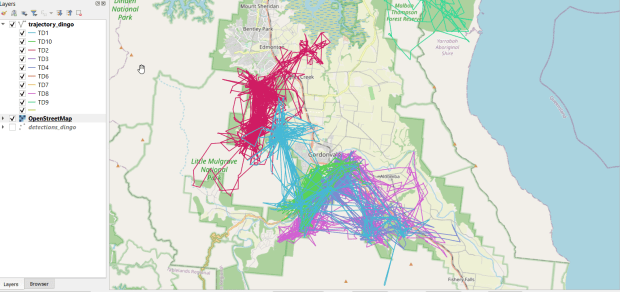
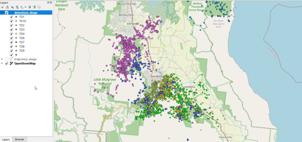
I describe how you can add and visualize this data in QGIS and ArcGIS Pro in the third and final part. Wildlife data comes packaged in a number of formats; in some cases you’ll find shapefiles or geodatabases that you can readily add and visualize, but more often than not the data is packaged in a plain CSV / TXT format. This requires you to plot the coordinates (X for longitude, Y for latitude) to create a dot map of the observations. Data files will often contain a number of individual animals, which can be uniquely identified with a tag ID, allowing you to symbolize the points by category so you have a different color or symbol for each individual. Alternatively, there might be separate data files for each individual, that you could add and symbolize differently. The files will contain either a sequential integer or a timestamp that indicates the order of the observations. With one field that indicates the order and another that identifies each individual, you can use a Points to Line or Points to Path tool to generate lines (tracks or trajectories) from the points (observations or detections).

You can see where dingos in Queensland, Australia are going in the screenshot below, which displays individual observation points, and the screenshot in the header of this post where the points were connected to form paths. I obtained the data from ZoaTrack and used QGIS for mapping. Check out the tutorial for details on how to find and map your favorite animals.

Dingo observations from ZoaTrack plotted in QGIS
Noise Complaint Kernels and Contours

Kernel Density and Contours in QGIS: Noisy NYC

In spatial analysis, kernel density estimation (colloquially referred to as a type of “hot spot analysis”) is used to explore the intensity or clustering of point-based events. Crimes, parking tickets, traffic accidents, bird sightings, forest fires, incidents of infections disease, anything that you can plot as a point at a specific period in time can be studied using KDE. Instead of looking at these features as a distribution of discrete points, you generate a raster that represents a continuous surface of values. You can either measure the density of the incidents themselves, or the concentration of a specific attribute that is tied to those incidents (like the dollar amount of parking tickets or the number of injuries in traffic accidents).

In this post I’ll demonstrate how to do a KDE analysis in QGIS, but you can easily implement KDE in other software like ArcGIS Pro or R. Understanding the inputs you have to provide to produce a meaningful result is more important than the specific tool. This YouTube video produced by the SEER Lab at the University of Florida helped me understand what these inputs are. They used the SAGA kernel tool within QGIS, but I’ll discuss the regular QGIS tool and will cover some basic data preparation steps when working with coordinate data. The video illustrates a KDE based on a weight, where there were single points that had a count-based attribute they wanted to interpolate (number of flies in a trap). In this post I’ll cover simple density based on the number of incidents (individual noise complaints), and will conclude by demonstrating how to generate contour lines from the KDE raster.

For a summary of how KDE works, take a look at the entry for “Kernel” in the Encyclopedia of Geographic Information Science (2007) p 247-248. For a fuller treatment, I always recommend Christopher Lloyd’s Spatial Data Analysis: An Introduction to GIS Users (2010) p 93-97 by Oxford Press. There’s also an explanation in the ArcGIS Pro documentation.

Data Preparation

I visited the NYC Open Data page and pulled up the entry for 311 Service Requests. When previewing the data I used the filter option to narrow the records down to a small subset; I chose complaints that were created between June 1st and 30th 2022, where the complaint type began with “Noise”, which gave me about 75,000 records (it’s a noisy town). Then I hit the Export button and chose one of the CSV formats. CSV is a common export option from open data portals; as long as you have columns that contain latitude and longitude coordinates, you will be able to plot the records. The NYC portal allows you to filter up front; other data portals like the ones in Philly and DC package data into sets of CSV files for each year, so if you wanted to apply filters you’d use the GIS or stats package to do that post-download. If shapefiles or geoJSON are provided, that will save you the step of having to plot coordinates from a CSV.

NYC Open Data 311 Service Requests

With the CSV, I launched QGIS, went to the Data Source Manager, and selected Delimited Text. Browsed for the file I downloaded, gave the layer a common sense name, and under geometry specified Point coordinates, and confirmed that the X field was my longitude column and the Y field was latitude. Ran the tool, and the points were plotted in the basic WGS 84 longitude / latitude system in degrees, which is the system the coordinates in the data file were in (generally a safe bet for modern coordinate data, but not always the case).

QGIS Add Delimited Text and Plot Coordinates

The next step was to save these plotted points in a file format that stores geometry and allows us to do spatial analysis. In doing that step, I recommend taking two additional ones. First, verify that all of the plotted data have coordinates – if there are any records where lat and long are missing, those records will be carried along into the spatial file but there will be no geometry for them, which will cause problems. I used the Select Features by Expression tool, and in the expression window typed “Latitude” is not null to select all the features that have coordinates.

QGIS Select by Expression

Second, transform the coordinate reference system (CRS) of the layer to a projected system that uses meters or feet. When we run the kernel tool, it will ask us to specify a radius for defining the density, as well as the size of the pixels for the output raster. Using degrees doesn’t make sense, as it’s hard for us to conceptualize distances in degrees, and they are not a constant unit of measurement. If you’ve googled around and read Stack Exchange posts or watched videos where a person says “You just have to experiment and adjust these numbers until your map looks Ok”, they were working with units in fractions of degrees. This is not smart. Transform the system of your layers!

I selected the layer, right clicked, Export, Save Selected Features As. The default output is a geopackage, which is fine. Otherwise you could select ESRI shapefile, both are vector formats that store geometry. For file name I browse … and save the file in a specific folder. Beside CRS I hit the globe button, and in the CRS Selector window typed NAD83 Long Island in the filter at the top, and at the bottom I selected the NAD83 / New York Long Island (ftUS) EPSG 2263 option system in the list. Every state in the US has one or more state plane zones that you can select for making optimal maps for that area, in feet or meters. Throughout the world, you could choose an appropriate UTM zone that covers your area in meters. For countries or continents, look for an equidistant projection (meters again).

QGIS Export – Save As

Clicked a series of Oks to create the new file. To reset my map window to match CRS of the new file, I selected that file, right clicked, Layer CRS, Set Project CRS from Layer. Removed my original CSV to avoid confusion, and saved my project.

QGIS Noise Complaints in Projected CRS

Kernel Density Estimation

Now our data is ready. Under the Processing menu I opened the toolbox and searched for kernel to find Heatmap (Kernel Density Estimation) under the Interpolation tools. The tool asks for an input point layer, and then a radius. The radius is used to define an area for calculating a local density estimate around each point. We can use a formula to determine an ideal radius; the hopt method seems to be commonly employed for this purpose.

To use the hopt formula, we need to know the standard distance for our layer, which measures the degree to which features are dispersed around the spatial mean or center of the distribution. A nice 3rd party plugin was created for calculating this. I went to the the plugins menu, searched for the Standard Distance plugin, and added it. Searched for it in the Processing toolbox and launched it. I provided my point layer for input, and specified an output file. The other fields are optional (if we were measuring an attribute of the points instead of the density of the points, we could specify the attribute as a weight column). The output layer consists of a circle where the center is the mean center of the distribution, and the circle represents the standard deviation. The attribute table contains one record, with the standard distance attribute of 36,046.18 feet (if no feature was created, the likely problem is you have records in the point file that don’t have geometry – delete them and try again).

Output from the Standard Distance Plugin

Knowing this, I used the hopt formula:

=((2/(3N))^0.25)SD

Where N is the number of features and SD is the standard distance. I used Excel to plug in these values and do the calculation.

((2/(374526))^0.25)36046.18 = 1971.33

Finally, I launched the heatmap kernel tool, specified my noise points as input, and the radius as 1,971 feet. The output raster size does take some experimentation. The larger the pixel size, the coarser or more general the resolution will be. You want to choose something that makes sense based on the size of the area, the number of points, and / or some other contextual information. Just like the radius, the units are based on the map units of your layer. If I type in 100 feet for Pixel X, I see I’ll have a raster with 1,545 rows and 1,565 columns. Change it to 200 feet, and I get 773 by 783. I’ll go with 200 feet (the distance between a “standard” numbered street block in midtown Manhattan). I kept the defaults for the other options.

QGIS Heatmap Kernel Density Estimation Window

The resulting raster was initially displayed in black and white. I opened the properties and symbology menu and changed the render type from Singleband gray to Singleband pseudocolor, and kept the default yellow to red scheme. Voila!

Kernel Density Estimate of NYC Noise Complaints June 2022

In June 2022 there were high clusters of noise complaints in north central Brooklyn, northern Manhattan, and the southwest portion of the Bronx. There’s a giant red hot spot in the north central Bronx that looks like the storm on planet Jupiter. What on earth is going on there? I flipped back to the noise point layer and selected points in that area, and discovered a single address where over 2,700 noise complaints about a loud party were filed on June 18 and 19! There’s also an address on the adjacent block that registered over 900 complaints. And yet the records do not appear to be duplicates, as they have different time stamps and closing dates. A mistake in coding this address, multiple times? A vengeful person spamming the 311 system? Or just one helluva loud party? It’s hard to say, but beware of garbage in, garbage out. Beyond this demo, I would spend more time investigating, would try omitting these complaints as outliers and run the heatmap tool again, and compare this output to different months. It’s also worth experimenting with the color classification scheme, and some different pixel sizes.

Kernel Results Zoomed In

Contour Lines

Another interesting way to visualize this data would be to generate contour lines based on the kernel output. I did a search for contour in the processing toolbox, and in the contour tool I provided the kernel noise raster as the input. For intervals between contour lines I tried 20 feet, and changed the attribute name to reflect what the contour represents: COMPLAINT instead of ELEV. Generated the new file, overlaid on top of the kernel, and now you can see how it represents the “elevation” of complaints.

Noise Complaint Kernel Density with Contour Lines

Switch the kernel off, symbolize the contours and add some labels, and throw the OpenStreetMap underneath, and now you can explore New York’s hills and valleys of noise. Or more precisely, the hills and valleys of noise complainers! In looking at these contours, it’s important to remember that they’re generated from the kernel raster’s grid cells and not from the original point layer. The raster is a generalization of the point layer, so it’s possible that if you look within the center of some of the denser circles you may not find, say, 340 or 420 actual point complaints. To generate a more precise set of contours, you would need to decrease the pixel size in the kernel tool (from say 200 feet to 100).

Noise Complaint Contours in Lower Manhattan, Northwest Brooklyn, and Long Island City

It’s interesting what you can create with just one set of points as input. Happy mapping!

Python API Code

Geocoding with the NYC Geoclient API and Python

Even though I’ve left New York, there are still occasions where I refer back to NYC resources in order to help students and faculty here with NYC-based research. Most recently I’ve revisited NYC DOITT’s Geoclient API for geocoding addresses, and I discovered a number of things have changed since I’ve last used it a few years ago. I’ll walk through my latest geocoding script in this post.

First and foremost: if you landed on this page because you’re trying to figure out how to get your Geoclient API key to work, the answer is:

&subscription-key=YOURKEYHERE

This replaces the old format that required you to pass an app id and key. I searched through two websites and scanned through hundreds of pages of documentation, only to find this solution in a cached Google search result, as the new docs don’t mention this change and the old docs still have the previous information and examples of the application ID and key. So – hopefully this should save you some hours of frustration.

I was working with someone who needed to geocode a subset of the city’s traffic violation data from the open data portal, as the data lacks coordinates. It’s also missing postal city names and ZIP Codes, which precludes using most geocoders that rely on this information. Even if we had these fields, I’ve found that many geocoders struggle with the hyphenated addresses used throughout Queens, and some work-around is needed to get matches. NYC’s geoclient is naturally able to handle those Queens addresses, and can use the borough name or code for locating addresses in lieu of ZIP Codes. The traffic data uses pseudo-county codes, but it’s easy to replace those with the corresponding borough codes.

The older documentation is still solid for illustrating the different APIs and the variables that are returned; you can search for a parsed or non-parsed street address, street intersections, places of interest or landmarks, parcel blocks and lots, and a few others.

I wrote some Python code that I’ve pasted below for geocoding addresses that have house numbers, street, and borough stored in separate fields using the address API, and if the house number is missing we try again by doing an intersection search, as an intersecting street is stored in a separate field in the traffic data. In the past I used a thin client for accessing the API, but I’m skipping that as it’s simpler to just build the URLs directly with the requests module.

The top of the script has the standard stuff: the name of the input file, the column locations (counting from zero) in the input file that contain each of the four address components, the base URL for the API, a time function for progress updates, reading the API key in from a file, and looping through the input CSV with the addressees to save the header row in one list and the records in a nested list. I created a list of fields that are returned from the API that I want to hold on to and add them to the header row, along with a final variable that records the results of the match. In addition to longitude and latitude you can also get xCoordinate and yCoordinate, which are in the NY State Plane Long Island (ft-US) map projection. I added a counts dictionary to keep track of the result of each match attempt.

Then we begin a long loop – this is a bit messy and if I had more time I’d collapse much of this into a series of functions, as there is repetitive code. I loop through the index and value of each record beginning with the first one. The loop is in a try / except block, so in the event that something goes awry it should exit cleanly and write out the data that was captured. We take the base url and append the address request, slicing the record to get the values for house, street, and borough into the URL. An example of a URL after passing address components in:

https://api.nyc.gov/geo/geoclient/v1/address.json?houseNumber=12345&street=CONEY ISLAND AVE&borough=BROOKLYN&subscription-key=KEYGOESHERE

Pass that URL to the requests module and get a response back. If an address is returned, the JSON resembles a Python dictionary, with ‘address’ as the key and the value as another dictionary with key value pairs of several variables. Otherwise, we get an error message that something was wrong with the request.

An address dictionary with sub-dictionaries returned by the NYC Geoclient
A successful address match returns an address dictionary, with a sub-dictionary of keys and values

The loop logic:

  • If the package contains an ‘address’ key, flatten to get the sub-dictionary
    • If ‘longitude’ is present as a key, a match is returned, get the relevant fields and append to the record
    • Else if the dictionary contains a ‘message’ key with a value that the house number was missing, do an intersection match
      • If the package contains an ‘intersection’ key, flatten to get the sub-dictionary
        • If ‘longitude’ is present as a key, a match is returned, get the relevant fields and append to the record
        • If not, there was no intersection match, just get the messages and append blanks for each value to the record
      • If not, an error was returned, capture the error and append blanks for each value to the record, and continue
    • If not, there was no address match, just get the messages and append blanks for each value to the record
  • If not, an error was returned, capture the error and append blanks for each value to the record, and continue

The API has limits of 2500 matches per minute and 500k per day, so after 2000 records I built in a pause of 15 seconds. Once the process finishes, successfully or not, the records are written out to a CSV file, header row first followed by the records. If the process bailed prematurely, the last record and its index are printed to the screen. This allows you to rerun the script where you left off, by changing the start index in the variables list at the top of the script from 0 to the last record that was read. When it comes time to write output, the previous file is appended rather than overwritten and the header row isn’t written again.

It took about 90 minutes to match a file of 25,000 records. I’d occasionally get an error message that the API key was bad for a given record; the error would be recorded and the script continued. It’s likely that there are illegal characters in the input fields for the address that end up creating a URL where the key parameter can’t be properly interpreted. I thought the results were pretty good; beyond streets it was able to recognize landmarks like large parks and return matched coordinates with relevant error messages (example below). Most of the flops were, not surprisingly, due to missing borough codes or house numbers.

Output from the NYC Geoclient
Output fields from the NYC Geoclient written to CSV

To use this code you’ll need to sign up for an NYC Developer API account, and then you can request a key for the NYC Geoclient service. Store the key in a text file in the same folder as the script. I’m also storing inputs and outputs in the same folder, but with a few functions from the os module you can manipulate paths and change directories. If I get time over the winter break I may try rewriting to incorporate this, plus functions to simplify the loops. An alternative to the API would be to download the LION street network geodatabase, and you could set up a local address locator in ArcGIS Pro. Might be worth doing if you had tons of matches to do. I quickly got frustrated with with the ArcGIS documentation and after a number of failed attempts I opted to use the Geoclient instead.

"""
Match addresses to NYC Geoclient using house number, street name, and borough
Frank Donnelly / GIS and Data Librarian / Brown University
11/22/2021 - Python 3.7
"""

import requests, csv, time

#Variables
addfile='parking_nov2021_nyc.csv' #Input file with addresses
matchedfile=addfile[:-4]+'_output.csv' #Output file with matched data
keyfile='nycgeo_key.txt' #File with API key
start_idx=0 #If program breaks, change this to pick up with record where you left off
#Counting from 0, positions in the CSV that contain the address info 
hous_idx=23
st_idx=24
boro_idx=21
inter_idx=25
base_url='https://api.nyc.gov/geo/geoclient/v1/'

def get_time():
    time_now = time.localtime() # get struct_time
    pretty_time = time.strftime("%m/%d/%Y, %H:%M:%S", time_now)
    return pretty_time

print('*** Process launched at', get_time())

#Read api key in from file
with open(keyfile) as key:
    api_key=key.read().strip()

records=[]

with open(addfile,'r') as infile:
    reader = csv.reader(infile)
    header = next(reader) # Capture column names as separate list
    for row in reader:
        records.append(row)

# Fields returned by the API to capture
# https://maps.nyc.gov/geoclient/v1/doc
fields=['message','message2','houseNumber','firstStreetNameNormalized',
        'uspsPreferredCityName','zipCode','longitude','latitude','xCoordinate',
        'yCoordinate']
header.extend(fields)
header.append('match_result')
datavals=len(fields)-2 # Number of fields that are not messages
counts={'address match':0, 'intersection match':0,
        'failed address':0, 'failed intersection':0,
        'error':0}

print('Finished reading data from', addfile)
print('*** Geocoding process launched at',get_time())

for i,v in enumerate(records[start_idx:]):
    try:
        data_url = f'{base_url}address.json?houseNumber={v[hous_idx]}&street={v[st_idx]}&borough={v[boro_idx]}&subscription-key={api_key}'
        response=requests.get(data_url)
        package=response.json()
        # If an address is returned, continue
        if 'address' in package:
            result=package['address']     
            # If longitude is returned, grab data
            if 'longitude' in result:
                for f in fields:
                    item=result.get(f,'')
                    v.append(item)
                v.append('address match')
                counts['address match']=counts['address match']+1
            # If there was no house number, try street intersection match instead
            elif 'message' in result and result['message']=='INPUT CONTAINS NO ADDRESS NUMBER' and v[inter_idx] not in ('',None):
                try:
                    data_url = f'{base_url}intersection.json?crossStreetOne={v[st_idx]}&crossStreetTwo={v[inter_idx]}&borough={v[boro_idx]}&subscription-key={api_key}'
                    response=requests.get(data_url)
                    package=response.json()
                    # If an intersection is returned, continue
                    if 'intersection' in package:
                        result=package['intersection']
                        # If longitude is returned, grab data
                        if 'longitude' in result:
                            for f in fields:
                                item=result.get(f,'')
                                v.append(item)
                            v.append('intersection match')
                            counts['intersection match']=counts['intersection match']+1
                        # Intersection match fails, append messages and blank values
                        else:
                            v.append(result.get('message',''))
                            v.append(result.get('message2',''))
                            v.extend(['']*datavals)
                            v.append('failed intersection')
                            counts['failed intersection']=counts['failed intersection']+1
                    # Error returned instead of intersection
                    else:
                        v.append(package.get('message',''))
                        v.append(package.get('message2',''))
                        v.extend(['']*datavals)
                        v.append('error')
                        counts['error']=counts['error']+1
                        print(package.get('message',''))
                        print('Geocoder error at record',i,'continuing the matching process...')
                except Exception as e:
                     print(str(e))
            # Address match fails, append messages and blank values
            else:
                v.append(result.get('message',''))
                v.append(result.get('message2',''))
                v.extend(['']*datavals)
                v.append('failed address')
                counts['failed address']=counts['failed address']+1
        # Error is returned instead of address
        else:
            v.append(package.get('message',''))
            v.append(package.get('message2',''))
            v.extend(['']*datavals)
            v.append('error')
            counts['error']=counts['error']+1
            print(package.get('message',''))
            print('Geocoder error at record',i,'continuing the matching process...')
        if i%2000==0:
            print('Processed',i,'records so far...')
            time.sleep(15)         
    except Exception as e:
        print(str(e))

# First attempt, write to new file, but if break happened, append to existing file
if start_idx==0:
    wtype='w' 
else:
    wtype='a'

end_idx=start_idx+i

with open(matchedfile,wtype,newline='') as outfile:
    writer = csv.writer(outfile, delimiter=',', quotechar='"',
                        quoting=csv.QUOTE_MINIMAL)
    if wtype=='w':
        writer.writerow(header)
        writer.writerows(records[start_idx:end_idx])
    else:
        writer.writerows(records[start_idx:end_idx])
print('Wrote',i+1,'records to file',matchedfile)
print('Final record written was number',i,':\n',v)
for k,val in counts.items():
    print(k,val)
print('*** Process finished at',get_time())

Map of Windham High Peak hike

From Survey Markers to GPS Coordinates

Here’s a fun post to close out the year. During GIS-based research consultations, I often help people understand the importance of coordinate reference systems (or spatial reference systems if you prefer, aka “map projections”). These systems essentially make GIS “work”; they are standards that allow you to overlay different spatial layers. You transform layers from one system to another in order to get them to align, perform specific operations that require a specific system, or preserve one aspect of the earth’s properties for a certain analysis you’re conducting or a map you’re making.

Wrestling with these systems is a conceptual issue that plays out when dealing with digital data, but I recently stumbled across a physical manifestation purely by accident. During the last week of October my wife and I rented a tiny home up in the Catskill Mountains in NY State, and decided to go for a day hike. The Catskills are home to 35 mountains known collectively as the Catskill High Peaks, which all exceed 3,500 feet in elevation. After consulting a thorough blog on upstate walks and hikes (Walking Man 24 7), we decided to try Windham High Peak, which was the closest mountain to where we were staying. We were rewarded with this nice view upon reaching the summit:

View from Summit of Windham High Peak

While poking around on the peak, we discovered a geodetic survey marker from 1942 affixed to the face of a rock. These markers were used to identify important topographical features, and to serve as control points in manual surveying to measure elevation; this particular marker (first pic below) is a triangulation marker that was used for that purpose. It looks like a flat, round disk, but it’s actually more like the head of a large nail that’s been driven into the rock. A short distance away was a second marker (second pic below) with a little arrow pointing toward the triangulation marker. This is a reference marker, which points to the other marker to help people locate it, as dirt or shrubbery can obscure the markers over time. Traditional survey methods that utilized this marker system were used for creating the first detailed sets of topographic maps and for establishing what the elevations and contours were for most of the United States. There’s a short summary of the history of the marker’s here, and a more detailed one here. NOAA provides several resources for exploring the history of the national geodetic system.

Triangulation Survey Marker

Triangulation Survey Marker

Reference Survey Marker

Reference Survey Marker

When we returned home I searched around to learn more about them, and discovered that NOAA has an app that allows you to explore all the markers throughout the US, and retrieve information about them. Each data sheet provides the longitude and latitude coordinates for the marker in the most recent reference system (NAD 83), plus previous systems that were originally used (NAD 27), a detailed physical description of the location (like the one below), and a list of related markers. It turns out there were two reference markers on the peak that point to the topographic one (we only found the first one). The sheet also references a distant point off of the peak that was used for surveying the height (the azimuth mark). There’s even a recovery form for submitting updated information and photographs for any markers you discover.

NA2038’DESCRIBED BY COAST AND GEODETIC SURVEY 1942 (GWL)
NA2038’STATION IS ON THE HIGHEST POINT AND AT THE E END OF A MOUNTAIN KNOWN
NA2038’AS WINDHAM HIGH PEAK. ABOUT 4 MILES, AIR LINE, ENE OF HENSONVILLE
NA2038’AND ON PROPERTY OWNED BY NEW YORK STATE. MARK, STAMPED WINDHAM
NA2038’1942, IS SET FLUSH IN THE TOP OF A LARGE BOULDER PROTRUDING
NA2038’ABOUT 1 FOOT, 19 FEET SE OF A LONE 10-INCH PINE TREE. U.S.
NA2038’GEOLOGICAL SURVEY STATION WINDHAM HIGH PEAK, A DRILL HOLE IN A
NA2038’BOULDER, LOCATED ON THIS SAME MOUNTAIN WAS NOT RECOVERED.

For the past thirty plus years or so we’ve used satellites to measure elevation and topography.  I used my new GPS unit on this hike; I still chose a simple, bare-bones model (a Garmin eTrex 10), but it was still an upgrade as it uses a USB connection instead of a clunky serial port. The default CRS is WGS 84, but you can change it to NAD 83 or another geographic system that’s appropriate for your area. By turning on the tracking feature you can record your entire route as a line file. Along the way you can save specific points as way points, which records the time and elevation.

Moving the data from the GPS unit to my laptop was a simple matter of plugging it into the USB port and using my operating system’s file navigator to drag and drop the files. One file contained the tracks and the other the way points, stored in a Garmin format called a gpx file (a text-based XML format). While QGIS has a number of tools for working with GPS data, I didn’t need to use any of them. QGIS 3.4 allows you to add gpx files as vector files. Once they’re plotted you can save them as shapefiles or geopackages, and in the course of doing so reproject them to a projected coordinate system that uses meters or feet. I used the field calculator to add a new elevation column to the way points to calculate elevation in feet (as the GPS recorded units in meters), and to modify the track file to delete a line; apparently I turned the unit on back at our house and the first line connected that point to the first point of our hike. By entering an editing mode and using the digitizing tool, I was able to split the features, delete the segments that weren’t part of the hike, and merge the remaining segments back together.

Original plot with line mistake

Original way points and track plotted in QGIS, with erroneous line

Using methods I described in an earlier post, I added a USGS topo map as a WMTS layer for background and modified the symbology of the points to display elevation labels, and voila! We can see all eight miles of our hike as we ascended from a base of 1,791 to a height of 3,542 feet (covering 1,751 feet from min to max). We got some solid exercise, were rewarded with some great views, and experienced a mix of old and new cartography. Happy New Year – I hope you have some fun adventures in the year to come!

Map of Windham High Peak hike

Stylized way points with elevation labels and track displayed on top of USGS topo map in QGIS

Python Geocoding Take 2 – US Addresses

Python Geocoding Take 1 – International Addresses I discussed my recent adventures with geocoding addresses outside the US. In contrast, there are countless options for batch geocoding addresses within the United States. I’ll discuss a few of those options here, but will focus primarily on the US Census Geocoder and a Python script I’ve written to batch match addresses using their API. The code and documentation is available on my lab’s resources page.

A Few Different Options

ESRI’s geocoding services allow you (with an account) to access their geocoding servers through tools in the ArcToolbox, or you can write a script and access them through an API. QGIS has a third-party plugin for accessing Google’s services (2500 records a day free) or the Open Streetmap. You can still do things the old fashioned way, by downloading geocoded street files and creating a matching service.

Alternatively, you can subscribe to any number of commercial or academic services where you can upload a file, do the matching, and download results. For years I’ve used the geocoding services at Texas A&M that allow you to do just that. Their rates are reasonable, or if you’re an academic institution and partner with them (place some links to their service on their website) you can request free credits for doing matches in batches.

The Census Geocoder and API, and a Python Script for Batch Geocoding

The Census Bureau’s TIGER and address files are often used as the foundational layers for building these other services, to which the service providers add refinements and improvements. You can access the Census Bureau’s services directly through the Census Geocoder, where you can match an address one at a time, or you can upload a batch of 1000 records. It returns longitude and latitude coordinates in NAD 83, and you can get names and codes for all the census geographies where the address is located. The service is pretty picky about the structure of the upload file (must be plain text, csv, with an id column and then columns with the address components in a specific order – with no other attributes allowed) but the nice thing is it requires no login and no key. It’s also public domain, so you can do whatever you want with the data you’ve retrieved. A tutorial for using it is available on our lab’s census tutorials page.

census geocoder

They also have an API with some basic documentation. You can match parsed and unparsed addresses, and can even do reverse geocoding. So I took a stab at writing a script to batch process addresses in text-delimited files (csv or txt). Unfortnately, the Census Geocoding API is not one of the services covered by the Python Geocoder that I mentioned in my previous post, but I did find another third party module called censusgeocode which provides a thin wrapper you can use. I incorporated that module into my Python 3 script, which I wrote as a function that takes the following inputs:

census_geocode(datafile,delim,header,start,addcol)
(str,str,str,int,list[int]) -> files

  • datafile – this is the name of the file you want to process (file name and extension). If you place the geocode_census_funct.py file in the same directory as your data file, then you just need to provide the name of the file. Otherwise, you need to provide the full path to the file.
  • delim – this is the delimiter or character that separates the values in your data file. Common delimiters includes commas ‘,’, tabs ‘t’, and pipes ‘|’.
  • header – here you specify whether your file has a header row, i.e. column names. Enter ‘y’ or ‘yes’ if it does, ‘n’ or ‘no’ if it doesn’t.
  • start – type 0 to specify that you want to start reading the file from the beginning. If you were previously running the script and it broke and exited for some reason, it provides an index number where it stopped reading; if that’s the case you can provide that index number here, to pick up where you left off.
  • addcol – provide a list that indicates the position number of the columns that contain the address components in your data file. For an unparsed address, you provide just one position number. For a parsed address, you provide 4 positions: address, city, state, and ZIP code. Whether you provide 1 or 4, the numbers must be supplied in brackets, as the function requires a Python list.

You can open the script in IDLE, run it to load it into memory, and then type the function with the necessary parameters in the shell to execute it. Some examples:

  • A tab-delimited, unparsed address file with a header that’s stored in the same folder as the script. Start from the beginning and the address is in the 2nd column: census_geocode('my_addresses.txt','t','y',0,[2])
  • A comma-delimited, parsed address file with no header that’s stored in the same folder as the script. Start from the beginning and the addresses are in the 2nd through 5th columns: census_geocode('addresses_to_match.csv',',','n',0,[2,3,4,5])
  • A comma-delimited, unparsed address file with a header that’s not in the same folder as the script. We ran the file before and it stopped at index 250, so restart there – the address is in the 3rd column: census_geocode('C:address_datadata1.csv',',','y',250,[3])

The beginning of the script “sets the table”: we read the address columns into variables, create the output files (one for matches, one for non-matches, and a summary report), and we handle whether or not there’s a header row. For reading the file I used Python’s CSV module. Typically I don’t use this module, as I find it’s much simpler to do the basic: read a line in, split it on a delimiter, strip whitespace, read it into a list, etc. But in this case the CSV module allows you to handle a wider array of input files; if the input data was a csv and there happened to be commas embedded in the values themselves, the CSV module easily takes care of it; if you ignore it, the parsing would get thrown off for that record.

Handling Exceptions and Server Errors

In terms of expanding my skills, the new things I had to learn were exception handling and control flows. Since the censusgeocoding module is a thin wrapper, it had no built in mechanism for retrying a match a certain number of times if the server timed out. This is an absolute necessity, because the census server often times out, is busy, or just hiccups, returning a generic error message. I had already learned how to handle crashes in my earlier geocoding experiments, where I would write the script to match and write a record one by one as it went along. It would try to do a match, but if any error was raised, it would exit that loop cleanly, write a report, and all would be saved and you could pick up where you left off. But in this case, if that server non-response error was returned I didn’t want to give up – I wanted to keep trying.

So on the outside there is a loop to try and do a match, unless any error happens, then exit the loop cleanly and wrap up. But inside there is another try loop, where we try to do a match but if we get that specific server error, continue: go back to the top of that for loop and try again. That loop begins with While True – if we successfully get to the end, then we start with the next record. If we get that server error we stay in that While loop and keep trying until we get a match, or we run out of tries (5) and write as a non-match.

error handling

In doing an actual match, the script does a parsed or unparsed match based on user input. But there was another sticking point; in some instances the API would return a matched result (we got coordinates!), but some of the objects that it returned were actually errors because of some java problem (failed to get the tract number or county name – here’s an error message instead!) To handle this, we have a for i in range loop. If we have a matched record and we don’t have a status message (that indicates an error) then we move along and grab all the info we need – the coordinates, and all the census geography where that coordinate falls, and write it out, and then that for loop ends with a break. But if we receive an error message we continue – go back to the top of that loop and try doing the match again. After 3 tries we give up and write no match.

Figuring all that out took a while – where do these loops go and what goes in them, how do I make sure that I retry a record rather than passing over it to the next one, etc. Stack Exchange to the rescue! Difference between continue, pass and break, returning to the beginning of a loop, breaking out of a nested loop, and retrying after an exception. The rest is pretty straightforward. Once the matching is done we close the files, and write out a little report that tells us how many matches we got versus fails. The Census Geocoder via the API is pretty unforgiving; it either finds a match, or it doesn’t. There is no match score or partial matching, and it doesn’t give you a ZIP Code or municipal centroid if it can’t find the address. It’s all or nothing; if you have partial or messy addresses or PO Boxes, it’s pretty much guaranteed that you won’t get matches.

There’s no limit on number of matches, but I’ve built in a number of pauses so I’m not hammering the server too hard – one second after each match, 5 seconds after every 1000 matches, a couple seconds before retrying after an error. Your mileage will vary, but the other day I did about 2500 matches in just under 2 hours. Their server can be balky at times – in some cases I’ve encountered only a couple problems for every 100 records, but on other occasions there were hang-ups on every other record. For diagnostic purposes the script prints every 100th record to the screen, as well as any problems it encountered (see pic below). If you launch a process and notice the server is hanging on every other record and repeatedly failing to get matches, it’s probably best to bail out and come back later. Recently, I’ve noticed fewer problems during off-peak times: evenings and weekends.

script_running

Wrap Up

The script and the documentation are posted on our labs resources page, for all to see and use – you just have to install the third party censusgeocode module before using it. When would you want to use this? Well, if you need something that’s free, this is a good choice. If you have batches in the 10ks to do, this would be a good solution. If you’re in the 100ks, it could be a feasible solution – one of my colleagues has confirmed that he’s used the script to match about 40k addresses, so the service is up to the task for doing larger jobs.

If you have less than a couple thousand records, you might as well use their website and upload files directly. If you’re pushing a million or more – well, you’ll probably want to set up something locally. PostGIS has a TIGER module that lets you do desktop matching if you need to go into the millions, or you simply have a lot to do on a consistent basis. The excellent book PostGIS in Action has a chapter dedicated to to this.

In some cases, large cities or counties may offer their own geocoding services, and if you know you’re just going to be doing matches for your local area those sources will probably have greater accuracy, if they’re adding value with local knowledge. For example, my results with NYC’s geocoding API for addresses in the five boroughs are better than the Census Bureau’s and is customized for local quirks; for example, I can pass in a borough name instead of a postal city and ZIP Code, and it’s able to handle those funky addresses in Queens that have dashes and similar names for multiple streets (35th st, 35th ave, 35th dr…). But for a free, public domain service that requires no registration, no keys, covers the entire country, and is the foundation for just about every US geocoding platform out there, the Census Geocoder is hard to beat.