In my previous post, I summarized several efforts to rescue and preserve US federal government datasets that are being removed from the internet. In this post, I’ll provide a basic primer on screen scraping with Python, which is what I’ve used to capture datasets in participating in the Data Rescue Project. Screen scraping can employed to many ends, such as capturing text on web pages so it can be analyzed, or taking statistics embedded in HTML tables and saving them in machine readable formats. In the context of this post, screen scraping is an approach for downloading data and documentation files stored on websites.
There are several benefits to using a scripting approach for this work. It saves you from the tedious task of clicking and downloading files one by one. The script serves as documentation for what you did, and allows you to easily repeat the process in the future, if the datasets continue to exist and are updated. A scripted, screen-scraping approach may not be best or necessary if the website and datasets are relatively small and simple, or conversely if the site is complicated and difficult to scrape given the technology it employs. In both cases, manual downloading may be quicker, especially with a team of volunteers. Furthermore, if it seems clear that the dataset or website are not going to be updated, or are going to vanish, then the benefit of repeating the process in the future is moot.
In this example, we’ll assume that screen scraping is the way to go, and we’ll use Python to do it. I’ll address a few alternatives to this approach at the end, the primary one being using an API if and when it’s available, and will share links to working code that colleagues and I have written to save datasets.
You should only apply these approaches to public, open data. Capturing restricted or proprietary information violates licenses, terms of service, and in some cases privacy constraints, and is not condoned by any of the rescue projects. Even if the data is public, bear in mind that scraping can put undue pressure on web servers. For large websites, plan accordingly by building pauses into the process, breaking up the work into segments, or running programs at non-peak times (overnight). When writing and testing scripts, don’t repeat the process over and over again on the entire website; run your tests on samples until you get everything working.
Screen Scraping Basics
The first step is to explore the website where the data is hosted, to identify the best pages to use as a source and determine the feasibility of the approach. Many websites will have feature rich, user friendly pages that make it easy to view extracts of data and visualize it, such as the NOAA climate website below.
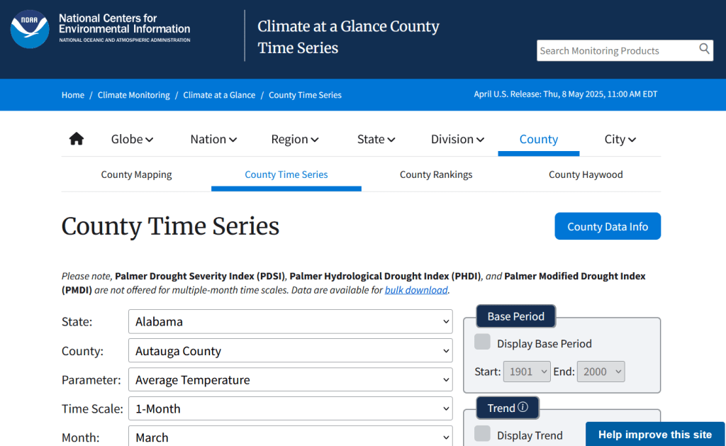
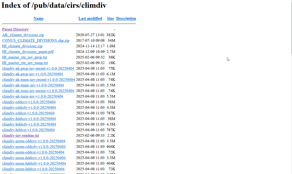
While easy to use, these pages can be complex and tedious to scrape. Always look for an option for bulk downloading datasets. They may lead you to a page sitting behind the scenes of the fancy website, such as the NOAA file directory below. Saving data from a page like this is fairly straightforward.
For the benefit of those of you who are not 1990s era people like myself and may not be familiar with working with HTML, the example below illustrates a simple webpage. With any browser, you can right click on a page and View the Source, to see the HTML code and stylesheets behind the page, which the browser processes and renders to display the site. HTML is a markup language where text is enclosed in tags that tell us something about the content within the tags, and which can be used for displaying the content in different ways. HTML is also hierarchical, so that content can be nested. For example, there is a head section that contains preliminary content about the page, and a body section that encloses the main content. Within the body there can be divisions, and anchor tags that represent links. In this example, one of these anchors is a link to a data file that we want to download.
<html>
<head>
    <title>Example Webpage</title>
</head>
<body>
    <div class='content'>
        <p>Paragraph with text.</p>
        <a href='https://www.page.gov/data.zip'/>
        <a href='https://www.page.gov/page.html'/>
    </div>
</body>
</html>
We can use Python to parse these tags and pull out desired content. There are four core modules I always use: Requests for downloading content, os for creating folders and working with paths, Beautiful Soup for screen scraping, and datetime for creating time stamps. In the code below, we begin by importing the modules and saving the url of the page we wish to scrape as a variable.
In most Python environments (unless you’ve modified some settings) it’s assumed that your current working directory is the folder where your Python script is stored. When you download files, they will automatically be stored in that folder. To keep things tidy, I always create a subfolder named with the date; I use the date function from datetime to retrieve today’s date, append that date to the word “downloaded-‘, and use the os module to create a subfolder with that name. If we run the program at a later date it will save everything in a new folder, rather than overwriting existing files.
import requests, os
from bs4 import BeautifulSoup as soup
from datetime import date

url='https://www.page.gov'

today = str(date.today())
outfolder='downloaded-'+today
if not os.path.exists(outfolder):
    os.makedirs(outfolder)

webpage=requests.get(url).content
soup_page=soup(webpage,'html.parser')
page_title = soup_page.title.text
container=soup_page.find('div',{'class':'content'})
links=container.findAll('a')
The final block in this example captures data from the website. We use requests to get the content stored at the url (the webpage), and then we pass this to Beautiful Soup, which parses all the HTML using their tags. Once parsed, we can retrieve specific objects. For example, we can save the page title (the text that appears in the heading of your browser for a particular site) as a variable. We also grab the section of the page that contains the links we want to capture by looking for a specific div or id tag. This isn’t strictly necessary for simple pages like this one, but speeds up processing for larger, more complex pages. Lastly, we can search through that specific container to find all the anchor tags, or links.
Once we have the links, we loop through and save the ones we want. My preference is to store them in a dictionary as key / value pairs, where the key is the name of the file, and the value is the file’s URL. We iterate through the links we saved, and with the soup we determine if the link has an ‘href’ attribute. If it does, we see if it ends with .zip, which is the data file. This skips any link that’s not a file we want, including links that go to other webpages as opposed to files. In practice, I provide a list of several file types here such as .zip, .csv, .txt, .xlsx, .pdf, etc to capture anything that could be data or documentation. If we find the zip, we split the link’s attributes from one string of text into a list of strings that are separated by the backslash, and grab the last element, which is the name of the file. Lastly, we add this to our datalinks dictionary; in this example, we’d have: {'data.zip':'https://www.page.gov/data.zip'}.
datalinks={}

for lnk in links:
    if 'href' in lnk.attrs:
        if lnk.attrs['href'].endswith(('.zip')):
            fname=lnk.attrs['href'].split('/')[-1]
            datalinks[fname]=lnk.attrs['href']
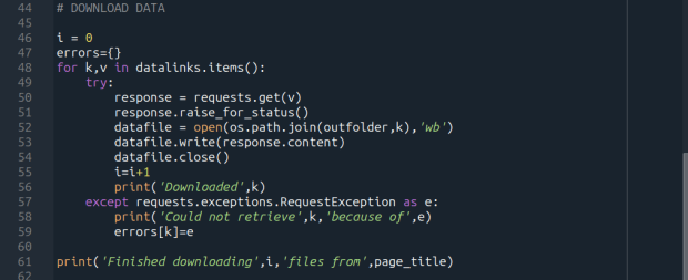
Time to download! We loop through each key (file name) and value (url) in our dictionary. We use the requests module to try and get the url (v), but if there’s a problem with the website or the link is invalid we bail out. If successful, we use the os module to go to our output folder and we supply the name of the file from the website (k) as the name of the file that we want to store on our computer. The ‘wb’ parameter specifies that we’re writing bytes to a file. I always like to keep count of the number of files I’ve done with an iterator (i) so I can print messages to a screen or a log file.
i = 0
for k,v in datalinks.items():
    try:
        response=requests.get(v)
        response.raise_for_status()
        dfile=open(os.path.join(outfolder,k),'wb')
        dfile.write(response.content)
        dfile.close()
        i=i+1
        print('Downloaded',k)
    except requests.exceptions.RequestException as e:
        print('Could not get',k,'because of',e)
print('Downloaded',i,'files from',page_title)
It’s important to save documentation too, so people can understand how the data was created and structured. In addition to saving pdf and text files, you can also save a vanilla copy of the website; I use a generic name with a date stamp. This saves the basic HTML text of the page, but not any images, documents, or styling. Which is usually good enough for providing documentation.
wfile = '_WEBPAGE-{}.html'.format(today)
writefile=open(os.path.join(outfolder,wfile),'wb')
writefile.write(webpage)
writefile.close()
As mentioned previously, you don’t want to place undue burden on the webserver. With the time module, you can use the sleep function and add a pause to your script for a fixed amount of time, usually at the end of a loop, or after your iterator has recorded a certain number of files. The random module allows you to supply a random time value within a range, if you want to vary the length of the pause.
import time
from random import randint

# Pause fixed amount
time.sleep(5)

# Pause random amount within a range
time.sleep(randint(10,20))
Screen Scraping Caveats
Those are the basics! Now here are the primary exceptions. The first problem is that links to files may not be absolute links that contain the entire path to a file. Sometimes they’re relative, containing a reference to just the subfolder and file. The requests module won’t be able to find these, so we have to take the extra step of building the full path, as in the example below. You can do this by identifying what the relative path starts with (unless they’re all relative and the same), and you create the absolute by adding (concatenating) the root url and the relative one contained in the soup.
    <div class='content'>
        <p>Paragraph with text.</p>
        <a href='/us/data.zip'/>
    </div>
url='https://www.page.gov'
datalinks={}
for lnk in links:
    if lnk.attrs['href'].endswith(('.zip')):
        if lnk.attrs['href'].startswith('/us/'):
            fname=lnk.attrs['href'].split('/')[-1]
            datalinks[fname]=url+lnk.attrs['href']
            ...
In other cases, a link to a data file may not lead directly to the file, but leads to another web page where that file is stored. We can embed another scraping block into a loop; retrieve and start scraping the main page, then once you find a link go to that page, and repeat retrieval and scraping. In these cases, it’s best to save these steps in a function, so you can call the function multiple times instead of repeating the same code.
<div class='content'>
        <p>Paragraph with text.</p>
        <a href='https://www.page.gov/us/'>
 </div>
Some websites will have dedicated pages where they embed a parameter in the url, such as codes for countries or states. If you know what these are, you can define them in a list, and iterate through that list by formatting the url to insert the code, and then scrape that page. If a page uses a unique integer as an ID and you know what the upper limit is, you can use for i in range(1,n) to step through each page (but make sure you handle exceptions, in case an integer isn’t used or is missing).
codes=['us','ca','mx']
url='https://www.page.gov/{}'
for c in codes:
    webpage=requests.get(url.format(c)).content
    soup_page=soup(webpage,'html.parser')
    ...
For complicated sites with several pages, you might not want to dump all the files into the same folder. Instead, as you iterate through pages, you can create a dedicated folder for that iteration. Using the example above, if there is a page for each country code, you can create a folder for that code and when writing files, use the path module to store files in that folder for that iteration.
codes=['us','ca','mx']
for c in codes:
    ...
    cfolder=os.path.join(outfolder,c)
        if not os.path.exists(cfolder):
            os.makedirs(cfolder)
    ...
    response=requests.get(v)
        response.raise_for_status()
        dfile=open(os.path.join(cfolder,k),'wb')
        dfile.write(response.content)
        dfile.close()
For websites with lots of files, or with a few big files, you may run out of memory during the download process and your script will go kaput. To avoid this, you can stream a file in chunks instead of trying to download it in one go. Use the request module’s iter_content function, and supply a reasonable chunk size in bytes (10000000 bytes is 10 MB).
...
try:
    with requests.get(v,stream=True) as response:
        response.raise_for_status()
        fpath=os.path.join(outfolder,k)
        with open(fpath,'wb') as writefile:
            for chunk in response.iter_content(chunk_size=10000000):
                writefile.write(chunk)
    i=i+1
    print('Downloaded',k)
except requests.exceptions.RequestException as e:
        print('Could not get',fname,'because of',e)
If you view the page source for a website, and don’t actually see the anchor links and file names in the HTML, you’re probably dealing with a page that employs JavaScript, which is a show stopper if you’re using Beautiful Soup. There may be a dropdown menu or option you have to choose first, in order to render the actual page (and you may be able to use the page parameters trick above, if the url on each page varies). But you may be stuck; instead of links, there may be download buttons you have to press or a dropdown menu option you have to choose in order to download the file.
One option would be to use a Python module called Selenium, which allows you to automate the process of using a web browser, to open a page, find a button, and click it. I’ve tried Selenium with some success, but find that it’s complex and clunky for screen scraping. It’s browser dependent (you’re automating the use of a browser, and they’re all different), and you’re forced to incorporate lots of pauses; waiting for a page to load before attempting to parse it, and dealing with pop up menus in the browser as you attempt to download multiple files, etc.
Another option that I’m not familiar with, and thus haven’t tried, would be to use JavaScript since that’s what the page uses. Most browsers have web developer console add-ons that allow you to execute snippets of JavaScript code in order to do something on a page. So some automation may be possible.
Using an API
You may be able to avoid scraping altogether if the data is made available via an API. With a REST API, you pass parameters into a base link to make a specific request. Using requests, you go to that URL, and instead of getting a web page you get the data that you’ve asked for, usually packaged in a JSON type object within your program (Python or another scripting language). Some APIs retrieve documents or dataset files, that you can stream and download as described previously. But most APIs for statistical data retrieve individual data records, which you would store in a nested list or dictionary and then write out to a CSV. The example below grabs the total population for four large cities in Rhode Island from 2020 decennial census public redistricting dataset.
import requests,csv

year='2020'
dsource='dec' # survey
dseries='pl' # dataset
cols='NAME,P1_001N' # variables
state='44' # geocodes for states
place='19180,54640,59000,74300' # geocodes for places
outfile='census_pop2020.csv'
keyfile='census_key.txt'

with open(keyfile) as key:
	api_key=key.read().strip()

base_url = f'https://api.census.gov/data/{year}/{dsource}/{dseries}'

# for sub-geography within larger geography - geographies must nest
data_url = f'{base_url}?get={cols}&for=place:{place}&in=state:{state}&key={api_key}'

response=requests.get(data_url)

popdata=response.json()
for record in popdata:
    print(record)

with open(outfile, 'w', newline='') as writefile:
    writer=csv.writer(writefile, quoting=csv.QUOTE_MINIMAL, delimiter=',')
    writer.writerows(popdata)
The benefit of an API is that it’s designed to retrieve machine readable data, and might be easier than scraping pages that have complex interfaces. The major downside is, if you’re forced to download individual records as opposed to entire files, the process can take a long time, to the point where it may be infeasible if the datasets are too large. It’s always worth checking to see if there is a bulk download option as that could be easier and more efficient (for example, the Census Bureau has an FTP site for downloading datasets in their entirety). Using an API also requires you to invest time in studying how it works, so you can build the appropriate links and ensure that you’re capturing everything.
Conclusion
Screen scraping will vary from website to website, but once you have enough examples it becomes easy to resample your code. You’ll always need to modify the Beautiful Soup step based on the structure of the individual pages, but the requests downloading step is more rote and may not require much modification. While I use Python, you can use other languages like R to achieve similar results.
Visit my library’s US Federal Government Data Backup GitHub for working examples of code that I and colleagues have used to capture datasets. In my programs I’ve added extra components, like writing a basic metadata file and error logs, which I haven’t covered in this post. The NOAA County at a Glance, IRS-SOI, and IMLS, scripts are basic examples, and the IMLS ones include some of the caveats I’ve described. The NOAA lake and sea level rise scripts are far more complex, and include cycling through many pages, creating multiple folders, streaming downloads, and encapsulating processes into functions. The USAID DHS Indicators scripts used APIs that retrieved files, while the USAID DHS SDR script used Selenium to step through a series of JavaScript pages.
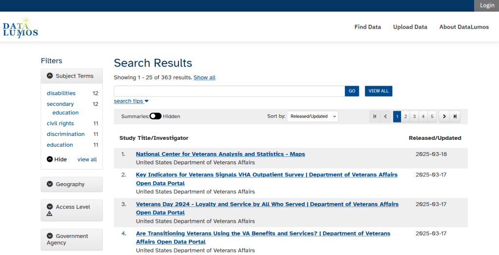
You’ll find scripts but no datasets in the GitHub repo due to file size limitations. If you’re a member of an institution that has access to GLOBUS, you can access the data files by following the instructions at the top of the page. Otherwise, we’ve contributed all of our datasets to DataLumos (except for the sea level rise data, I’m working with another university to host that).




You must be logged in to post a comment.