articles

Interesting reports or articles published

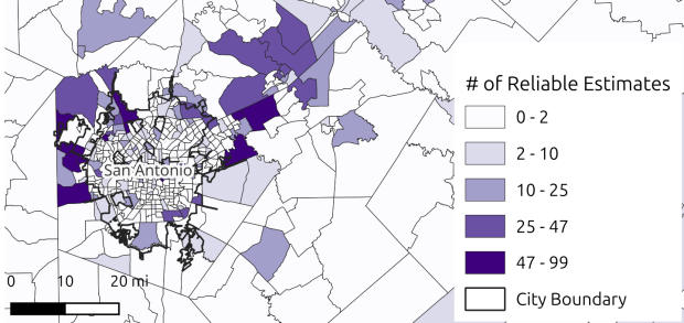
Map of San Antonio Showing Reliable Estimates by census tract

Comparing 5-year ACS Estimates Over Time

My article on comparing American Community Survey (ACS) estimates over time was published earlier this month. It will take another 6 to 12 months before it’s slotted into a actual volume and issue, but until then it’s available online via the link in this citation:

Donnelly, F. P. (2026). The Feasibility of Comparing 5-Year American Community Survey Estimates Over Time. Journal of the American Planning Association, 1–14. https://doi.org/10.1080/01944363.2026.2709860

Unfortunately it’s not open access; if you don’t have a subscription, you can read the article in the publisher’s e-pub platform; this link only works for the first 100 clicks, then it’s kaput. I’ll eventually post the pre-published version of the article on this website, as I can freely share it. Much of the summary data from the research and the scripts I wrote for processing and analyzing the data are available on GitHub.

Background

The idea for the paper sprang from my work helping graduate students compare estimates over time when making maps in GIS. I wrote a post about these early experiences, where I described the fairly involved process we had to take to prepare and assess the estimates, only to discover that statistically they were not comparable (you couldn’t discern actual change from sample variability), or if they were comparable they were too imprecise to be useful. I wondered, how feasible is it to compare estimates over time – is going through all of these steps ever worthwhile?

To answer this question, I chose 25 detailed tables that captured a broad range of variables and represented basic, fundamental tables that many researchers would likely use. These tables included over 300 individual variables. For example, table B01001 included 49 variables: total population, total population that was male and that was female, and then 5-year age cohorts by sex (male population aged 0-4, male population aged 5-9, etc). I chose 19 geographic summary levels that represented the most essential geographies, from the nation down to census block groups. I compared estimates for these variables from the 2010-2014 to the 2015-2019 ACS for approximately 400,000 individual geographic areas; I chose these two 5-year periods as they do not overlap, and they are drawn from the same geographic vintage (2010) so I would not have to account for geographic boundary changes that occur with each decennial census.

ACS TABLES INCLUDED IN THE STUDY

Table IDTable NameVariablesObservations (M)% Total
B01001Sex by Age4919.918.0%
B01002Median Age by Sex31.21.1%
B02001Race104.13.7%
B03002Hispanic or Latino Origin by Race218.57.7%
B05002Place of Birth by Nativity and Citizenship*15†2.82.5%
B07204Geographical Mobility in the Past Year*19†3.53.2%
B08006Workers by Means of Transportation to Work*17†3.12.8%
B11001Household Type (Including Living Alone)93.73.3%
B13002Women Who Had a Birth in the Past 12 Months*193.53.2%
B14001School Enrollment by Level of School*101.81.7%
B15002Sex by Educational Attainment3514.212.9%
C17002Ratio of Income to Poverty Level83.22.9%
B19001Household Income (Dollars)176.96.2%
B19013Median Household Income (Dollars)10.40.4%
B19083Gini Index of Income Inequality*10.20.2%
B23025Employment Status72.82.6%
C24030Sex by Industry for Employed Civilians29†11.810.6%
B25002Occupancy Status31.21.1%
B25003Tenure31.21.1%
B25010Average Household Size of Occupied Housing Units31.21.1%
B25063Gross Rent24†9.78.8%
B25064Median Gross Rent (Dollars)10.40.4%
B25070Gross Rent as a Percentage of Household Income114.54.0%
B25077Median Home Value (Dollars)10.40.4%
B26001Group Quarters Population*10.20.2%

* Data for block groups and tribal block groups is not published for this table
† Value represents a subset of the total variables in the table; some variables were excluded

I opted against randomly sampling the variables, which would have allowed me to statistically analyze the results and make “firmer” assumptions. The primary audience for the paper is a practitioner-based one, for whom it’s more meaningful to have complete results for all geographies, for all or most variables in tables that people commonly use. The variables I chose also represent relatively broad swaths of the population. A random sample would have yielded many variables for small populations from disparate tables, which would be of limited interest.

I calculated change and percent change for each pair of estimates from the two time periods. I applied the test for significant difference, to determine if the estimates from both time periods were truly different from another, or if any difference was likely the result of sampling variation. If the estimates were significantly different, I calculated the coefficient of variation, to determine how reliable the estimates were. I summarized the results by variable, table, and geographic summary level. Ultimately, I had a dataset with 110.5 million individual data points that represented change for a variable between two time periods for a given place, of which 107.5 mil­lion were distinct (i.e. variables included in more than one table were only counted once).

Results

The results were surprising. Approximately 90% of the time, estimates from the two time periods were not statistically different from each other, and thus could not be reliably compared to compute change over time. The estimates that were significantly different were of low precision approximately 90% of the time (a CV value higher than 30). In short, it’s usually not worth investing the effort that’s involved with comparing two, consecutive 5-year period ACS estimates over time.

That being said, there are exceptions. Not surprisingly, the larger a population was, or the larger the sample size, the more likely it was that the estimates would be comparable and reliable. For the nation as a whole, estimates were comparable about 94% of the time, and of those that were comparable, estimates were of reliable precision about 98% of the time (a CV value less than 30). Both of these values fall to 73% for states, to 28% and 34% for counties, and 12% and 6% for census tracts. When considering all estimates regardless of geography, variables that represented large segments of the population were also more comparable and reliable. For example, estimates for the total population, median home value, population not enrolled in school, and workers 16 years and older were comparable 25% to 30% of the time and reliable 22% to 33% of the time.

There were some interesting divergences. Estimates for workers who take various forms of public transit to work ranked low in terms of being statistically comparable, but of the estimates that were comparable, they tended to be the most reliable. While this population is small or zero in many parts of the country, it is large and highly clustered in dense urban areas, so when the values are comparable they are of high precision. So if you were doing research in New York City or Chicago, you would have good estimates to work with (but not so if you were looking at all tracts / places / ZCTAs in New York State or Illinois).

Beyond the relationship between population and sample size, areas or populations that experienced a large degree of growth or decline were also more likely to be comparable and reliable, as these large shifts outweighed any sample noise. These two time periods experienced dramatic growth in home value (adjusted for inflation) and decline in unemployment. Median home value was consistently ranked as one of the most comparable and reliable estimates, while the unemployed labor force was ranked as one of the most comparable (despite the fact that this population is relatively small). The map in the header of this post depicts census tracts in and around San Antonio, TX. Rapidly growing exurban tracts tended to have a higher number of reliable estimates (CV values less than 30).

As a data librarian, I was equally interested in the means to the end, as a large part of my mission is to support students and faculty with this process. During the data collection and analysis phase, I wrote a post that provided tips on working with big(ger) datasets when your computing power is limited to your laptop. I relied on a PostgreSQL database to efficiently store the data and generate the calculations, and I had to be thoughtful in how to use Python so that I didn’t run out of memory, eschewing popular tools that make things easy in favor of approaches that were more efficient, and using SQL and Python in tandem to do the work that each was best suited for.

While the ACS isn’t well suited for short-term historical comparisons, it remains a valuable and indispensable dataset. Its strength is that it gives us a detailed snapshot of our present circumstances, at a fine degree of geographic and temporal resolution that is unmatched by any other US government dataset. We should not confuse shortcomings with the data with calls to curtail or eliminate it. The current administration’s attempts to sabotage the federal statistical system are detrimental to our country’s economic and social well being. As data practitioners we need to support and protect our nation’s datasets, while collaborating with agencies to improve them.


US Census Data ALA Tech Report

ALA Tech Report on Using Census Data for Research

I have written a new report that’s just been released: US Census Data: Concepts and Applications for Supporting Research, was published as the May / June 2022 issue of the American Library Association’s Library and Technology Reports. It’s available for purchase digitally or in hard copy from the ALA from now through next year. It will also be available via EBSCOhost as full text, sometime this month. One year from now, the online version will transition to become a free and open publication available via the tech report archives.

The report was designed to be a concise primer (about 30 pages) for librarians who want to be knowledgeable with assisting researchers and students with finding, accessing, and using public summary census data, or who want to apply it to their own work as administrators or LIS researchers. But I also wrote it in such a way that it’s relevant for anyone who is interested in learning more about the census. In some respects it’s a good distillation of my “greatest hits”, drawing on work from my book, technical census-related blog posts, and earlier research that used census data to study the distribution of public libraries in the United States.

Chapter Outline

  1. Introduction
  2. Roles of the Census: in American society, the open data landscape, and library settings
  3. Census Concepts: geography, subject categories, tables and universes
  4. Datasets: decennial census, American Community Survey, Population Estimates, Business Establishments
  5. Accessing Data: data.census.gov, API with python, reports and data summaries
  6. GIS, historical research, and microdata: covers these topics plus the Current Population Survey
  7. The Census in Library Applications: overview of the LIS literature on site selection analysis and studying library access and user populations

I’m pleased with how it turned out, and in particular I hope that it will be used by MLIS students in data services and government information courses.

Although… I must express my displeasure with the ALA. The editorial team for the Library Technology Reports was solid. But once I finished the final reviews of the copy edits, I was put on the spot to write a short article for the American Libraries magazine, primarily to promote the report. This was not part of the contract, and I was given little direction and a month at a busy time of the school year to turn it around. I submitted a draft and never heard about it again – until I saw it in the magazine last week. They cut and revised it to focus on a narrow aspect of the census that was not the original premise, and they introduced errors to boot! As a writer I have never had an experience where I haven’t been given the opportunity to review revisions. It’s thoroughly unprofessional, and makes it difficult to defend the traditional editorial process as somehow being more accurate or thorough compared to the web posting and tweeting masses. They were apologetic, and are posting corrections. I was reluctant to contribute to the magazine to begin with, as I have a low opinion of it and think it’s deteriorated in recent years, but that’s a topic for a different discussion.

Stepping off the soapbox… I’ll be attending the ALA annual conference in DC later this month, to participate on a panel that will discuss the 2020 census, and to reconnect with some old colleagues. So if you want to talk about the census, you can buy me some coffee (or beer) and check out the report.

A final research and publication related note – the map that appears at the top of my post on the distribution of US public libraries from several years back has also made it into print. It appears on page 173 of The Argument Toolbox by K.J. Peters, published by Broadview Press. It was selected as an example of using visuals for communicating research findings, making compelling arguments in academic writing, and citing underlying sources to establish credibility. I’m browsing through the complimentary copy I received and it looks excellent. If you’re an academic librarian or a writing center professional and are looking for core research method guides, I would recommend checking it out.

NYC and NYMA Pop Change Graph 2000 to 2019

New York’s Population and Migration Trends in the 2010s

The Weissman Center for International Business at Baruch College just published my paper, “New York’s Population and Migration Trends in the 2010s“, as part of their Occasional Paper Series. In the paper I study population trends over the last ten years for both New York City (NYC) and the greater New York Metropolitan Area (NYMA) using annual population estimates from the Census Bureau (vintage 2019), county to county migration data (2011-2018) from the IRS SOI, and the American Community Survey (2014-2018). I compare NYC to the nine counties that are home to the largest cities in the US (cities with population greater than 1 million) and the NYMA to the 13 largest metro areas (population over 4 million) to provide some context. I conclude with a brief discussion of the potential impact of COVID-19 on both the 2020 census count and future population growth. Most of the analysis was conducted using Python and Pandas in Jupyter Notebooks available on my GitHub. I discussed my method for creating rank change grids, which appear in the paper’s appendix and illustrate how the sources and destinations for migrants change each year, in my previous post.

Terminology

  • Natural increase: the difference between births and deaths
  • Domestic migration: moves between two points within the United States
  • Foreign migration: moves between the United States and a US territory or foreign country
  • Net migration: the difference between in-migration and out-migration (measured separately for domestic and foreign)
  • NYC: the five counties / boroughs that comprise New York City
  • NYMA: the New York Metropolitan Area as defined by the Office of Management and Budget in Sept 2018, consists of 10 counties in NY State (including the 5 NYC counties), 12 in New Jersey, and one in Pennsylvania
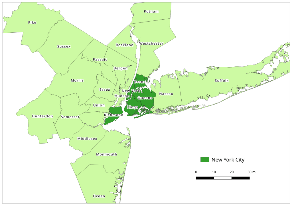
Map of the New York Metropolitan Area
The New York-Newark-Jersey City, NY-NJ-PA Metropolitan Area

Highlights

  • Population growth in both NYC and the NYMA was driven by positive net foreign migration and natural increase, which offset negative net domestic migration.
  • Population growth for both NYC and the NYMA was strong over the first half of the decade, but population growth slowed as domestic out-migration increased from 2011 to 2017.
  • NYC and the NYMA began experiencing population loss from 2017 forward, as both foreign migration and natural increase began to decelerate. Declines in foreign migration are part of a national trend; between 2016 and 2019 net foreign migration for the US fell by 43% (from 1.05 million to 595 thousand).
  • The city and metro’s experience fit within national trends. Most of the top counties in the US that are home to the largest cities and many of the largest metropolitan areas experienced slower population growth over the decade. In addition to NYC, three counties: Cook (Chicago), Los Angeles, and Santa Clara (San Jose) experienced actual population loss towards the decade’s end. The New York, Los Angeles, and Chicago metro areas also had declining populations by the latter half of the decade.
  • Most of NYC’s domestic out-migrants moved to suburban counties within the NYMA (representing 38% of outflows and 44% of net out-migration), and to Los Angeles County, Philadelphia County, and counties in Florida. Out-migrants from the NYMA moved to other large metros across the country, as well as smaller, neighboring metros like Poughkeepsie NY, Fairfield CT, and Trenton NJ. Metro Miami and Philadelphia were the largest sources of both in-migrants and out-migrants.
  • NYC and the NYMA lack any significant relationships with other counties and metro areas where they are net receivers of domestic migrants, receiving more migrants from those places than they send to those places.
  • NYC and the NYMA are similar to the cities and metros of Los Angeles and Chicago, in that they rely on high levels foreign migration and natural increase to offset high levels of negative domestic migration, and have few substantive relationships where they are net receivers of domestic migrants. Academic research suggests that the absolute largest cities and metros behave this way; attracting both low and high skilled foreign migrants while redistributing middle and working class domestic migrants to suburban areas and smaller metros. This pattern of positive foreign migration offsetting negative domestic migration has characterized population trends in NYC for many decades.
  • During the 2010s, most of the City and Metro’s foreign migrants came from Latin America and Asia. Compared to the US as a whole, NYC and the NYMA have slightly higher levels of Latin American and European migrants and slightly lower levels of Asian and African migrants.
  • Given the Census Bureau’s usual residency concept and the overlap in the onset the of COVID-19 pandemic lock down with the 2020 Census, in theory the pandemic should not alter how most New Yorkers identify their usual residence as of April 1, 2020. In practice, the pandemic has been highly disruptive to the census-taking process, which raises the risk of an under count.
  • The impact of COVID-19 on future domestic migration is difficult to gauge. Many of the pandemic destinations cited in recent cell phone (NYT and WSJ) and mail forwarding (NYT) studies mirror the destinations that New Yorkers have moved to between 2011 and 2018. Foreign migration will undoubtedly decline in the immediate future given pandemic disruptions, border closures, and restrictive immigration policies. The number of COVID-19 deaths will certainly push down natural increase for 2020.

census_paper_wcib_ops

An Overview of Census Datasets and Census API Examples

This month’s post is a bit shorter, as I have just two announcements I wanted to share about some resources I’ve created.

First, I’ve written a short technical paper that’s just been published as part of the Weissman Center of International Business’ Occasional Papers Series. Exploring US Census Datsets: A Summary of Surveys and Sources provides an overview of several different datasets (decennial census, American Community Survey, Population Estimates Program, and County Business Patterns) and sources for accessing data. The paper illustrates basic themes that are part of all my census-related talks: the census isn’t just the thing that happens every ten years but is an ecosystem of datasets updated on an on-going basis, and there are many sources for accessing data which are suitable for different purposes and designed for users with varying levels of technical skill. In some respects this paper is a super-abridged version of my book, designed to serve as an introduction and brief reference.

Second, I’ve created a series of introductory notebooks on GitHub that illustrate how to use the Census Bureau’s API with Python and Jupyter Notebooks. I designed these for a demonstration I gave at NYU’s Love Data Week back on Feb 10 (the slides for the talk are also available in the repo). I structured the talk around three examples. Example A demonstrates the basics of how the API works along with some best practices, such as defining your variables at the top and progressively building links to retrieve data. It also illustrates the utility of using these technologies in concert, as you can pull data into your script and process and visualize it in one go. I also demonstrate how to retrieve lists of census variables and their corresponding metadata, which isn’t something that’s widely documented. Example B is a variation of A, extended by adding an API key and storing data in a file immediately after retrieval. Example C introduces more complexity, reading variables in from files and looping through lists of geographies to make multiple API calls.

Since I’ve written a few posts on the census API recently, I went back and added an api tag to group them together, so you can access them via a single link.

census api example

Define census API variables, build links, and retrieve data

Net Out-Migration from the NY Metro Area to Other Metro Areas 2011-2015

Recent Migration Trends for New York City and Metro

The Baruch GIS lab crew just published a paper: New Yorkers on the Move: Recent Migration Trends for the City and Metro Area. The paper (no. 15 Feb 2018) is part of the Weissman Center for International Business Occasional Paper Series, which focuses on New York City’s role in the international and domestic economy.

Findings

We analyzed recent population trends (2010 to 2016) in New York City and the greater metropolitan area using the US Census Bureau’s Population Estimates to study components of population change (births, deaths, domestic and international migration) and the IRS Statistics of Income division’s county to county migration data to study domestic migration flows.

Here are the main findings:

  1. The population of New York City and the New York Metropolitan Area increased significantly between 2010 and 2016, but annually growth has slowed due to greater domestic out-migration.
  2. Compared to other large US cities and metro areas, New York’s population growth depends heavily on foreign immigration and natural increase (the difference between births and deaths) to offset losses from domestic out-migration.
  3. Between 2011 and 2015 the city had few relationships where it was a net receiver of migrants (receiving more migrants than it sends) from other large counties. The New York metro area had no net-receiver relationships with any major metropolitan area.
  4. The city was a net sender (sending more migrants than it received) to all of its surrounding suburban counties and to a number of large urban counties across the US. The metro area was a net sender to metropolitan areas throughout the country.

For the domestic migration portion of the analysis we were interested in seeing the net flows between places. For example, the NYC metro area sends migrants to and receives migrants from the Miami metro. What is the net balance between the two – who receives more versus who sends more?

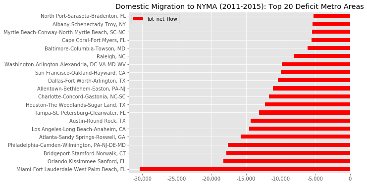
The answer is: the NYC metro is a net sender to most of the major metropolitan areas in the country, and has no significant net receiver relationships with any other major metropolitan area. For example, for the period from 2011 to 2015 the NYC metro’s largest net sender relationship was with the Miami metro. About 88,000 people left the NYC metro for metro Miami while 58,000 people moved in the opposite direction, resulting in a net gain of 30,000 people for Miami (or in other words, a net loss of 30k people for NYC). The chart below shows the top twenty metros where the NYC metro had a deficit in migration (sending more migrants to these areas than it received). A map of net out-migration from the NYC metro to other metros appears at the top of this post. In contrast, NYC’s largest net receiver relationship (where the NYC metro received more migrants than it sent) was with Ithaca, New York, which lost a mere 300 people to the NYC metro.

All of our summary data is available here.

domestic migration to NYMA 2011-2015: top 20 deficit metro areas

Process

For the IRS data we used the county to county migration SQLite database that Janine meticulously constructed over the course of the last year, which is freely available on the Baruch Geoportal. Anastasia employed her Python and Pandas wizardry to create Jupyter notebooks that we used for doing our analysis and generating our charts, all of which are available on github. I used an alternate approach with Python and the SQLite and prettytable modules to generate estimates independently of Anastasia, so we could compare the two and verify our numbers (we were aggregating migration flows across years and geographies from several tables, and calculating net flows between places).

One of our goals for this project was to use modern tools and avoid the clunky use of email. With the Jupyter notebooks, git and github for storing and syncing our work, and ShareLaTeX for writing the paper, we avoided using email for constantly exchanging revised versions of scripts and papers. Ultimately I had to use latex2rtf to convert the paper to a word processing format that the publisher could use. This post helped me figure out which bibliography packages to choose (in order for latex2rtf to interpret citations and references, you need to use the older natbib & bibtex combo and not biblatex & biber).

If you are doing similar research, Zillow has an excellent post that dicusses the merits of the different datasets. There are also good case studies on Washington DC and Philadelphia that employ the same datasets.

Article on the History of the US Census

I’ve been cranking away on my census book these past few months. I’m almost finished revising the preface and chapter 1 to submit as part of the book proposal review process, and a rough draft of chapter 2 is also complete.

I wrote a short piece on the history of the US census while I was doing background research last fall. It was recently published in Metropolitics, which is an on-line academic journal that specializes in short pieces on cities, urban politics, and urban economics. The journal was originally created in Paris as Metropolitiques, and a separate English-language version with a New York-based editorial board was created more recently. Each version is published independently and a select number of articles are translated from one version and published in the other, giving it a unique international flair in terms of content and contributors. A new article in the English version is published every Tuesday.

I wrote the piece as a lead-in to the 2020 census, which we’re starting to hear more about in the news. After spending a decade of research on creating new and improved categories for the race question, the OMB and White House decided not to accept the Bureau’s proposal and thus we’re keeping the same categories from 2010 and 2000. Meanwhile, the Justice Department is lobbying for a adding a citizenship question, which already appears in the American Community Survey and has not appeared in the short form of the decennial census since 1950. Read the article and follow the links to the references to see what the repercussions could be. The questions and categories must be finalized by March 31st…