When I’m making global thematic maps, I usually turn to Natural Earth. They provide country polygons and boundary lines, as well as features like cities and rivers, at several different scales. I always reference it in workshops that I teach, including the 2-week GIS Institute that I participated in earlier this month. It’s a solid, free data source and a good example for illustrating how scale and generalization work in cartography. It’s a “natural choice”, as they provide boundaries that depict the way the world actually looks.
I also discussed aesthetics and map design during the Institute. What if you don’t necessarily care about representing the boundaries exactly the way they are? If you rely on the map reader’s knowledge of the relative shape of the countries and their position on the globe, and you employ good labeling, you can choose boundaries that are more artistic and fun (provided that your only goal is making a basic thematic map and it’s not being published in a stodgy journal).
Project Linework is part of Something About Maps, an excellent blog by Daniel Huffman. The project consists of different series of public domain boundary files that have been generalized to provide interesting and visually attractive alternatives to standard features. The gallery contains a sample image and brief description of each series, including details on geographic coverage. Most of the series cover just North America or select portions of the world.
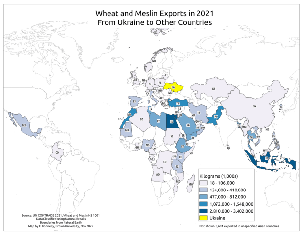
The three I’ll mention below are global in coverage. They come in shapefile and geojson formats, are projected in World Gall Stereographic (ESRI 54016), and include line and polygon coverages. The attribute tables have fields for ISO country codes, which are standard unique identifiers that allow for table joins for thematic mapping. I took my map of Wheat and Meslin Exports from Ukraine from an earlier post to create the following examples.
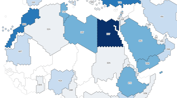
With the Wargames series, the world has been rendered using the little hexagon grids familiar to many war board gamers, and plenty of non-war gamers for that matter (think Settlers of Catan). Hexes are a an alternative to grids for determining adjacency.
Project Linework: Wargames
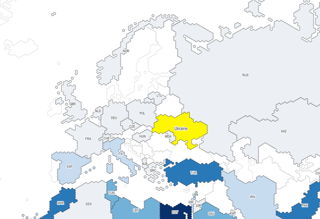
Moriarty Hand is a more whimsical interpretation. It was drawn by hand by tracing line work from Natural Earth. The end result is more organic compared to Wargames. It comes in two scales, small and large (with an example of the latter below):
Project Linework: Moriarty Hand
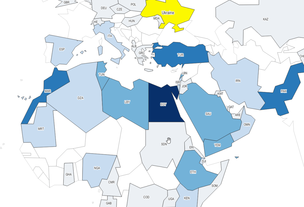
My personal favorite is 1981. It’s inspired by the basic polygon shapes that you would have seen in early computer graphics. When I was little I remember loading a DOS-based atlas program from a floppy disk, and slowly panning across a CGA monochrome screen as the machine chunked away to render countries that looked like these. Good if you’re looking for a retro vibe.
I’ve been receiving more questions about geospatial data sources as the semester draws to a close. I’ll describe some sources that I haven’t used extensively before in the next couple of posts, beginning with data on bilateral trade: imports and exports between countries. We’ll look at the IMF’s Direction of Trade Statistics (DOTS) and the UN’s COMTRADE database. Both sources provide web-based portals, APIs, and bulk downloading. I’ll focus on the portals.
IMF Direction of Trade Statistics
IMF DOTS provides monthly, quarterly, and annual import and export data, represented as total dollar values for all goods exchanged. The annual data goes back to 1947, while the monthly / quarterly data goes back to 1960. All countries that are part of the IMF are included, plus a few others. Data for exports are published on a Free and On Board (FOB) price basis, while imports are published on a Cost, Insurance, Freight (CIF) price basis. Here are definitions for each term, quoted directly from the OECD’s Statistical Glossary:
The f.o.b. price (free on board price) of exports and imports of goods is the market value of the goods at the point of uniform valuation, (the customs frontier of the economy from which they are exported). It is equal to the c.i.f. price less the costs of transportation and insurance charges, between the customs frontier of the exporting (importing) country and that of the importing (exporting) country.
The c.i.f. price (i.e. cost, insurance and freight price) is the price of a good delivered at the frontier of the importing country, including any insurance and freight charges incurred to that point, or the price of a service delivered to a resident, before the payment of any import duties or other taxes on imports or trade and transport margins within the country.
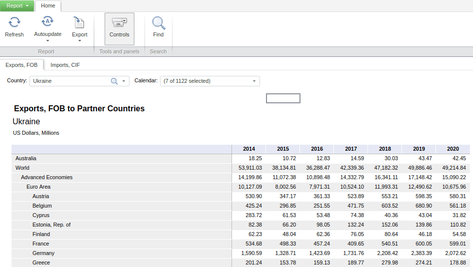
There are a few different ways to browse and search for data. Start with the Data Tables tab at the top, and Exports and Imports by Areas and Countries. The default table displays monthly exports by region and country for the entire world (you could switch to imports by selecting the Imports CIF tab beside the Export sFOB tab). Hitting the Calendar dropdown allows you to change the date range and frequency. Hitting the Country dropdown lets you select a specific region or country. In the example below, I’ve changed the calendar from months to years, and the country to Ukraine. By doing so, the table now depicts the total US dollar value of exports and imports between Ukraine and all other countries. The Export button at the top allows you to save the report in a number of formats, Excel being the most data friendly option.
IMF DOTS Basic Report – Total Value of Exports from Ukraine, Last Five Years
While this is the quickest option, it comes with some downsides; the biggest one is that there are no unique identifiers for the countries, which is important if you wanted to join this table to a GIS vector file for mapping, or another country-level table in a database.
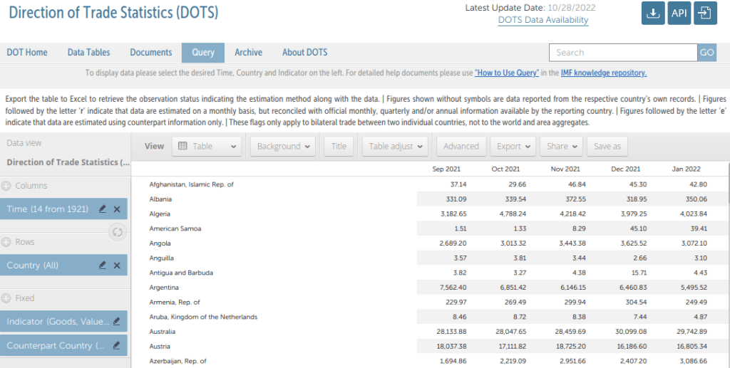
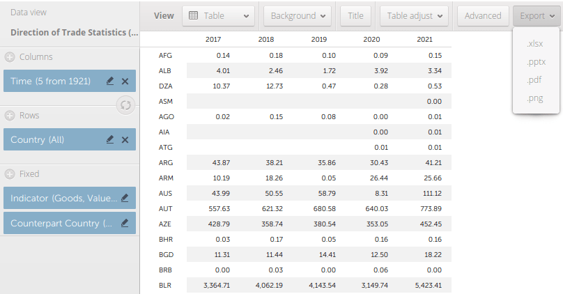
A better approach is to return to the home page and use the Query tab, which allows you to get a unique identifier and filter out countries and regions that are not of interest.
DOTS Query Tab
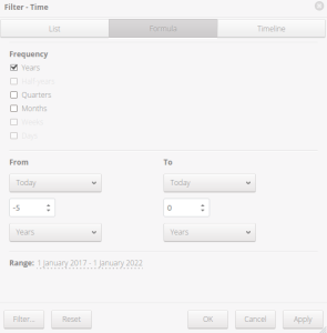
Under Columns, select the time frame and interval. For example, check Years for Frequency at the top, and change the dropdowns at the bottom from Months to Years. From -5 to 0 would give you the last five years in ascending order.
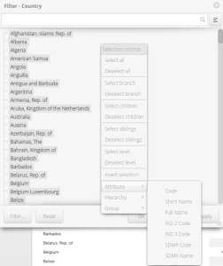
Rows allows you to filter out countries or regions that you don’t want to see in the results. You can also change the attribute that is displayed. Once the menu is open, right click in an empty area and choose Attribute. Here you can choose a variant country name, or an ISO country code. ISO codes are commonly used for uniquely identifying countries.
Indicator lets you choose Exports (FOB), Imports (CIF or FOB), or Trade Balance, all in US dollars.
Counterpart country is the country or region that you want to show trade for, such as Ukraine in our previous example.
The tabs along the top allow you to produce graphs instead of a table (View – Table), to pivot the table (Adjust), and calculate summaries like sums or averages (Advanced).
Export to produce an Excel file. By choosing the ISO codes you’ll lose the country names, but you can join the result to another country data table or shapefile and grab the names from there.
Modify Time
Modify Rows – Country – Change Attribute
DOTS Modified Table to Export: Total Value of Exports from Ukraine Last Five Years
UN COMTRADE
If you want data on the exchange of specific goods and services, quantities in addition to dollar values, and exchanges beyond simple imports and exports, then the UN’s COMTRADE database will be your source. You need to register to download data, but you can generate previews without having to log in. There is an extensive wiki that describes how to use the different database tools, and summaries of technical terms that you need to know for extracting and interpreting the data. You’ll need some understanding of the different systems for classifying commodities and goods. Your options (the links that follow lead to documentation and code lists) are: the Harmonized Classification System (HC), the Standard Industrial Trade Classification (SITC), and the Broad Economic Categories (BEC). What’s the difference? Here are some summaries, quoted directly from a UN report on the BEC:
The HS classification is maintained by the World Customs Organization. Its main purpose is to classify goods crossing the border for import tariffs or for application of some non-tariff measures for safety or health reasons. The HS classification is revised on a five-year cycle (p. 18)
The original SITC was designed in the 1950s as a tool for collection and dissemination of international merchandise trade statistics that would help in establishing internationally comparable trade statistics. By its introduction in 1988, the HS took over as collection and dissemination tool, and SITC was thereon used mostly as an analytical tool. (p. 19)
The Classification by Broad Economic Categories (BEC) is an international product classification. Its main purpose is to provide a set of broad product categories for the analysis of trade statistics. Since its adoption in 1971, statistical offices around the world have used BEC to report trade statistics in a concise and meaningful way (p. iii). The broad economic categories of BEC include all subheadings of the HS classification. Therefore, the total trade in terms of HS equals the total trade of the goods side of BEC. (p. 18)
In short, go with the BEC if you’re interested in high-level groupings, or the HS if you need detailed subdivisions. The SITC would be useful if you need to go further back in time, or if it facilitates looking at certain subdivisions or groupings that the other systems don’t capture.
From COMTRADE’s homepage, I suggest leaving the defaults in place and doing a basic, preliminary search for all global exports for the most recent year, so you can see basic output on the next screen. Then you can apply filters for a narrower search.
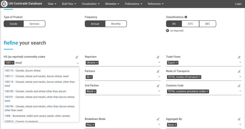
For example, let’s look at annual exports of wheat from Ukraine to other countries. Under the HS filter, remove the TOTAL code. Start typing wheat, and you’ll see various product categories: 6-digit codes are the most specific, while 4-digit codes are broader groups that encapsulate the 6-digit categories. We’ll choose wheat and meslin 1001. We’ll select Ukraine as the Reporter (the country that supplied the statistics and represents the origin point), and for the 1st partner we’ll choose All to get a list of all countries that Ukraine exported wheat to. The 2nd partner country we’ll leave as World (alternatively, you would add specific countries here if you wanted to know if there were intermediary nations between the origin and destination).
UN COMTARDE Refine Search with Filters
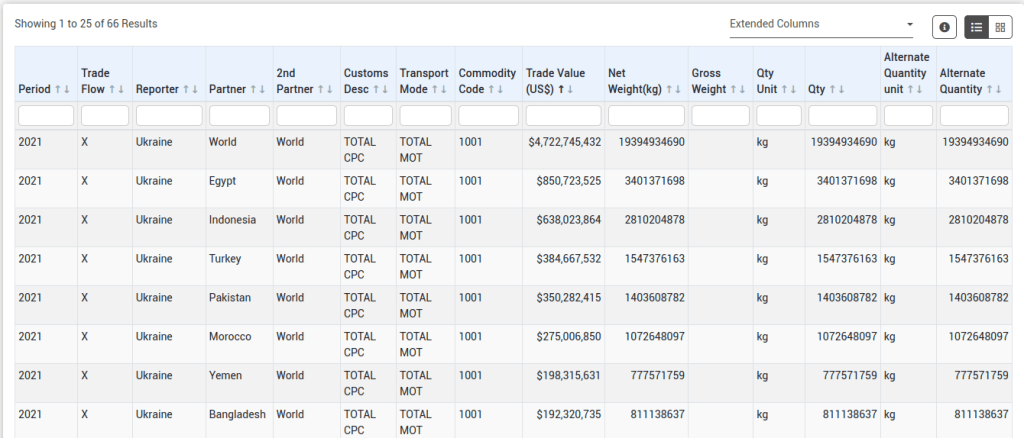
Hit Preview to see the results. You can click on a heading to sort by dollar value, weight, or country name. Like IMF DOTS, UN COMTRADE measures dollar amounts of exports as FOB and imports as CIF. At this point, you would need to log in to download the data as a CSV (creating an account is free). You would also need to be logged in if you generated an extract that has more than 500 records, otherwise the results will be truncated. You could always copy and paste data for shorter extracts directly from the screen to a spreadsheet, but you wouldn’t get any of the extra metadata fields that come with download, like ISO Country Codes and the classification codes for goods and merchandise.
COMTRADE Filtered Results – Exports of Wheat and Meslin from Ukraine 2021Data Exported from COMTRADE to CSV with Identifiers
Mapping
For data from either source, if you wanted to map it you’d need to have a data table where there is one row for each country with columns of attributes, and with one column that has the ISO country code to serve as a unique identifier. Save the data table in an Excel file or as a table in a database. Download a country shapefile from Natural Earth. Add the shapefile and data table to a project and join them using the ISO code. Natural Earth shapefiles have several different ISO code columns that represent nations, sovereigns, and parent – child relationships; be sure you select the right one. Data table records that represent regions or groupings of countries (i.e. the EU, ASEAN, sum of smaller countries per continent not enumerated, etc.) will fall out of the dataset, as they won’t have a matching feature in the country shapefile. The map at the top of this post was created in QGIS, using COMTRADE and Natural Earth.
I’m working on a project where I needed to generate a list of all the administrative subdivisions (i.e. states / provinces, counties / departments, etc) and their ID codes for several different countries. In this post I’ll demonstrate how I accomplished this using the Geonames API and Python. Geonames (https://www.geonames.org/) is a gazetteer, which is a directory of geographic features that includes coordinates, variant place names, and identifiers that classify features by type and location. Geonames includes many different types of administrative, populated, physical, and built-environment features. Last year I wrote a post about gazetteers where I compared Geonames with the NGA Geonet Names Server, and illustrated how to download CSV files for all places within a given country and load them into a database.
In this post I’ll focus on using an API to retrieve gazetteer data. Geonames provides over 40 different REST API services for accessing their data, all of them well documented with examples. You can search for places by name, return all the places that are within a distance of a set of coordinates, retrieve all places that are subdivisions of another place, geocode addresses, obtain lists of centroids and bounding boxes, and much more. Their data is crowd sourced, but is largely drawn from a body of official gazetteers and directories published by various countries.
This makes it an ideal source for generating lists of administrative divisions and subdivisions with codes for multiple countries. This information is difficult to find, because there isn’t an international body that collates and freely provides it. ISO 3166-1 includes the standard country codes that most of the world uses. ISO 3166-2 includes codes for 1st-level administrative divisions, but ISO doesn’t freely publish them. You can find them from various sources; Wikipedia lists them and there are several gist and github repos with screen scraped copies. The US GNA is a more official source that includes both ISO 3166 1 and 2. But as far as I know there isn’t a solid source for codes below the 1st level divisions. Many countries create their own systems and freely publish their codes (i.e. ANSI FIPS codes in the US, INSEE COG codes in France), but that would require you to tie them altogether. GADM is the go to source for vector-based GIS files of country subdivisions (map at the top of this post for example). For some countries they include ISO division codes, but for others they don’t (they do employ the HASC codes from Statoids, but it’s not clear if these codes are still being actively maintained) .
Geonames to the rescue – you can browse the countries on the website to see the country and 1st level admin codes (see image below), but the API will give us a quick way to obtain all division levels. First, you have to register to get an API username – it’s free – and you’ll tack that username on to the end of your requests. That gives you 20k credits per day, which in most instances equates with 1 request per credit. I recommend downloading one of their prepackaged country files first, to give you a sense for how the records are structured and what attributes are available. A readme file that describes all of the available fields accompanies each download.
1st Level Admin Divisions for Dominica from the Geonames website
My goal was to get all administrative divisions – names and codes and how the divisions nest within each other – for all of the countries in the French-speaking Caribbean (countries that are currently, or formerly, overseas territories of France). I also needed to get place names as they’re written in French. I’ll walk through my Python script that I’ve pasted below.
import requests,csv
from time import strftime

ccodes=['BL','DM','GD','GF','GP','HT','KN','LC','MF','MQ','VC']
fclass='A'
lang='fr'
uname='REQUEST FROM GEONAMES'

#Columns to keep
fields=['countryId','countryName','countryCode','geonameId','name','asciiName',
        'alternateNames','fcode','fcodeName','adminName1','adminCode1',
        'adminName2','adminCode2','adminName3','adminCode3','adminName4','adminCode4',
        'adminName5','adminCode5','lng','lat']
fcode=fields.index('fcode')

#Divisions to keep
divisions=['ADM1','ADM2','ADM3','ADM4','ADM5','PCLD','PCLF','PCLI','PCLIX','PCLS']

base_url='http://api.geonames.org/searchJSON?'

def altnames(names,lang):
    "Given a dict of names, extract preferred names for a given language"
    aname=''
    for entry in names:
        if 'isPreferredName' in entry.keys() and entry['lang']==lang:
            aname=entry.get('name')
        else:
            pass
    return aname

places=[]
tossed=[]

for country in ccodes:
    data_url = f'{base_url}?name=*&country={country}&featureClass={fclass}&lang={lang}&style=full&username={uname}'
    response=requests.get(data_url)
    data=response.json() #total retrieved and results in list of dicts
    gnames=response.json()['geonames'] #create list of dicts only
    gnames.sort(key=lambda e: (e.get('countryCode',''),e.get('fcode',''),
                               e.get('adminCode1',''),e.get('adminCode2',''),
                               e.get('adminCode3',''),e.get('adminCode4',''),
                               e.get('adminCode5','')))
    for record in gnames:
        r=[]
        for f in fields:
            item=record.get(f,'')
            if f=='alternateNames' and f !='':
                aname=altnames(item,'en')
                r.append(aname)
            else:
                r.append(item)
        if r[fcode] in divisions: #keep certain admin divs, toss others
            places.append(r)
        else:
            tossed.append(r)

filetoday=strftime('%Y_%m_%d')
outfile='geonames_fwi_adm_'+filetoday+'.csv'

writefile=open(outfile,'w', newline='', encoding='utf8')
writer=csv.writer(writefile, delimiter=",", quotechar='"',quoting=csv.QUOTE_NONNUMERIC)
writer.writerow(fields) #header row
writer.writerows(places)
writefile.close()

print(len(places),'records written to file',outfile)
First, I identify all of the variables I need: the two-letter ISO codes of the countries, a list of the Geonames attributes that I want to keep, the two-letter language code, and the specific feature type I’m interested in. There are different features codes classified with a single letter, and a number of subtypes below that. Feature class A is for records that represent administrative divisions, and within that class I needed records that represented the country as a whole (PCL codes) and its subdivisions (ADM codes). There are several different place name variables that include official names, short forms, and an ASCII form that only includes characters found in the Latin alphabet used in English. The language code that you pass into the url will alter these results, but you still have the option to obtain preferred place names from an alternate languages field. The admin codes I’m retrieving are the actual admin codes; you can also opt to retrieve the unique Geonames integer IDs for each admin level, if you wanted to use these for bridging places together (not necessary in my case).
There are a few different approaches for achieving this goal. I decided to use the Geonames full text search, where you search for features by name (separate APIs for working with hierarchies for parent and child entities are another option). I used an asterisk as a wildcard to retrieve all names, and the other parameters to filter for specific countries and feature classes. At the end of the base url I added JSON for the search; if you leave this off the records are returned as XML.
base_url='http://api.geonames.org/searchJSON?'
My primary for loop loops through each country, and passes the parameters into the data url to retrieve the data for that country: I pass in country code, feature class A, and French as the language for the place names. It took me a while to figure out that I also needed to add style=full to retrieve all of the possible info that’s available for a given record; the default is to capture a subset of basic information, which lacked the admin codes I needed.
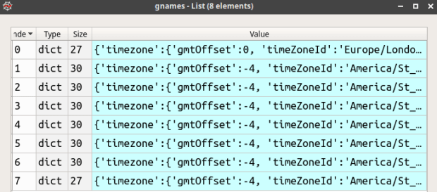
I use the Python Requests module to interact with the API. Geonames returns two objects in JSON: an integer count of the total records retrieved, and another JSON object that essentially represents a list of python dictionaries, where each dictionary contains all the attributes for a record as a series of key and value pairs where the key is the attribute name (see examples below). I create a new gnames variable to isolate just this list, and then I sort the list based on how I want the final output to appear; by country and by admin codes, so that like-levels of admin codes are grouped together. The trick of using lamba to sort nested lists or dictionaries is well documented, but one variation I needed was to use the dictionary get method. Some features may not have five levels of admin codes; if they don’t then there is no key for that attribute, and using the simple dict[key] approach returns an error in those cases. Using dict.get(key,”) allows you to pass in a default value if no key is present. I provide a blank string as a placeholder, as ultimately I want each record to have the same number of columns in the output and need the attributes to line up correctly.
Records returned from Geonames as a list, where each list item is a dictionary of key / value pairs for a given place
Example of an individual list item, a dictionary of key / value pairs for the Parish of Charlotte, a 1st order admin division of Saint-Vincent-et-les-Grenadines. Variable names are keys.
Once I have records for the first country, I loop through them and choose just the attributes that I want from my field list. The attribute name is the key, I get the associated value, but if that key isn’t present I insert an empty string. In most cases the value associated with a key is a string or integer, but in a few instance it’s another container, as in the case of alternate names which is another list of dictionaries. If there are alternate names I want to pull out a preferred name in English if one exists. I handle this with a function so the loop looks less cluttered. Lastly, if this record represents an admin division or is a country-level record then I want to keep it, otherwise I append it to a throw-away list that I’ll inspect later.
Once the records returned for that country have been processed, we move on to the next country and keep appending records to the main list of places (image below). When we’re done, we write the results out to a CSV file. I write the list of fields out first as my header row, and then the records follow.
Final list called places that contains records for all admin divisions for specific countries and feature classes, where items are sublists that represent each place
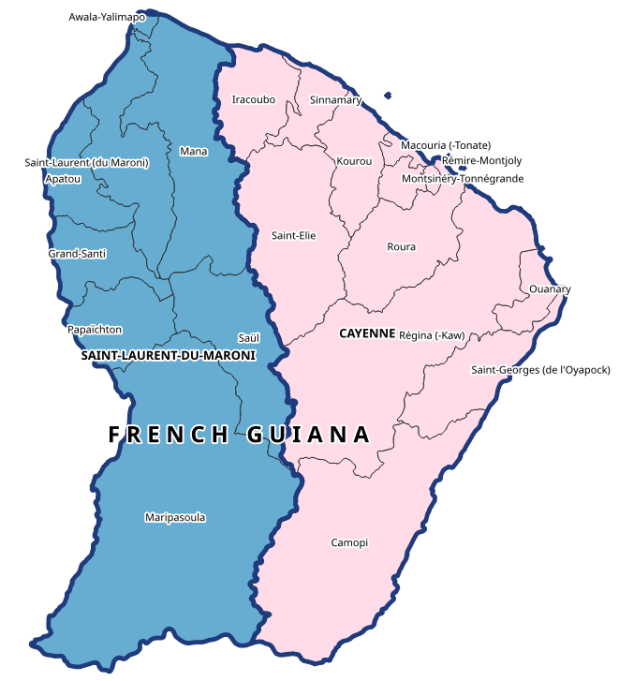
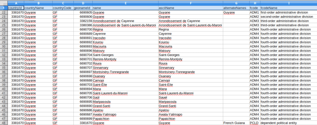
Overall I think this approach worked well, but there are some small caveats. A number of the countries I’m studying are not independent, but are dependencies of France. For dependent countries, their 1st and sometimes even 2nd level subdivision codes appear identical to their top-level country code, as they represent a subdivision of an independent country (many overseas territories are departments of France). If I need to harmonize these codes between countries I may have to adjust the dependencies. The alternate English places names always appear for the country-level record, but usually not below that. I think I’d need to do some additional tweaking or even run a second set of requests in English if I wanted all the English spellings; for example in French many compound place names like Saint-Paul are separated by a hyphen, but in English they’re separated by a space. Not a big deal in my case as I was primarily interested in the alternate spellings for countries, i.e. Guyane versus French Guiana. See the final output below for Guyane; these subdivision codes are from INSEE COG, which are the official codes used by the French government for identifying all geographic areas for both metropolitan France and overseas departments and collectivities.
1st half of CSV file imported into spreadsheet, records showing admin divisions of Guyane / French Guiana
2nd half of CSV file imported into spreadsheet, records showing admin codes and hierarchy of divisions for Guyane / French Guiana
Two final things to point out. First, my script lacks any exception handling, since my request is rather small and the API is reliable. If I was pulling down a lot of data I would replace my main for loop with a try and except block to handle errors, and would capture retrieved data as the process unfolds in case some problem forces a bail out. Second, when importing the CSV into a spreadsheet or database, it’s important to import the admin codes as text, as many of them have leading zeros that need to be preserved.
This example represents just the tip of the iceberg in terms of things you can do with Geonames APIs. Check it out!


You must be logged in to post a comment.