When aggregating small census geographies to larger ones (census tracts to neighborhoods for example) when you’re working with American Community Survey (ACS) data, you need to sum estimates and calculate new margins of error. This is straightforward for most estimates; you simply sum them, and take the square root of the sum of squares for the margins of error (MOEs) for each estimate that you’re aggregating. But what if you need to group and summarize derived estimates like means or medians? In this post, I’ll demonstrate how to calculate mean household income by aggregating ZCTAs to United Hospital Fund neighborhoods (UHF), which is a type of public health area in NYC created by aggregating ZIP Codes.
I’m occasionally asked how to summarize median household income from tracts to neighborhood-like areas. You can’t simply add up the medians and divide them, the result would be completely erroneous. Calculating a new median requires us to sort individual household-level records and choose the middle-value, which we cannot do as those records are confidential and not public. There are a few statistical interpolation methods that we can use with interval data (number of households summarized by income brackets) to estimate a new median and MOE, but the calculations are rather complex. The State Data Center in California provides an excellent tutorial that demonstrates the process, and in my new book I’ll walk through these steps in the supplemental material.
While a mean isn’t as desirable as a median (as it can be skewed by outliers), it’s much easier to calculate. The ACS includes tables on aggregate income, including the sum of all income earned by households and other population group (like families or total population). If we sum aggregate household income and number of households for our small geographic areas, we can divide the total income by total households to get mean income for the larger area, and can use the ACS formula for computing the MOE for ratios to generate a new MOE for the mean value. The Census Bureau publishes all the ACS formulas in a detailed guidebook for data users, and I’ll cover many of them in the ACS chapter of my book (to be published by the end of 2019).
Calculating a Derived Mean in Excel
Let’s illustrate this with a simple example. I’ve gathered 5-year 2017 ACS data on number of households (table B11001) and aggregate household income (table B19025) by ZCTA, and constructed a sheet to correlate individual ZCTAs to the UHF neighborhoods they belong to. UHF 101 Kingsbridge-Riverdale in the Bronx is composed of just two ZCTAs, 10463 and 10471. We sum the households and aggregate income to get totals for the neighborhood. To calculate a new MOE, we take the square root of the sum of squares for each of the estimate’s MOEs:
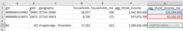
Calculate margin of error for new sum
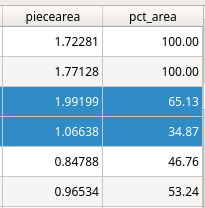
To calculate mean income, we simply divide the total aggregate household income by total households. Calculating the MOE is more involved. We use the ACS formula for derived ratios, where aggregate income is the numerator of the ratio and households is the denominator. We multiply the square of the ratio (mean income) by the square of the MOE of the denominator (households MOE), add that product to the square of the MOE of the numerator (aggregate income MOE), take the square root, and divide the result by the denominator (households):
=(SQRT((moe_ratio_numerator^2)+(ratio^2*moe_ratio_denominator^2))/ratio_denominator)
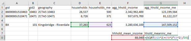
Calculate margin of error for ratio (mean income)
The 2013-2017 mean household income for UHF 101 is $88,040, +/- $4,223. I always check my math using the Cornell Program on Applied Demographic’s ACS Calculator to make sure I didn’t make a mistake.
This is how it works in principle, but life is more complicated. When I downloaded this data I had number of households by ZCTA and aggregate household income by ZCTA in two different sheets, and the relationship between ZCTAs and UHFs in a third sheet. There are 42 UHF neighborhoods and 211 ZCTAs in the city, of which 182 are actually assigned to UHFs; the others have no household population. I won’t go into the difference between ZIP Codes and ZCTAs here, as it isn’t a problem in this particular example.
Tying them all together would require using the ZCTA in the third sheet in a VLOOKUP formula to carry over the data from the other two sheets. Then I’d have to aggregate the data to UHF using a pivot table. That would easily give me sum of households and aggregate income by UHF, but getting the MOEs would be trickier. I’d have to square them all first, take the sum of these squares when pivoting, and take the square root after the pivot to get the MOEs. Then I could go about calculating the means one neighborhood at a time.
Spreadsheet-wise there might be a better way of doing this, but I figured why do that when I can simply use a database? PostgreSQL to the rescue!
Calculating a Derived Mean in PostgreSQL
In PostgreSQL I created three empty tables for: households, aggregate income, and the ZCTA to UHF relational table, and used pgAdmin to import ZCTA-level data from CSVs into those tables (alternatively you could use SQLite instead of PostgreSQL, but you would need to have the optional math module installed as SQLite doesn’t have the capability to do square roots).
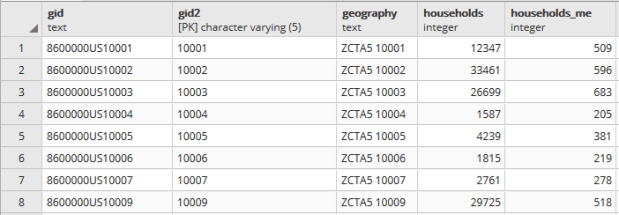
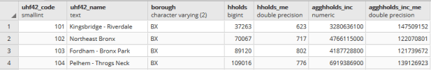
Portion of households table. A separate aggregate household income table is structured the same way, with income stored as bigint type.
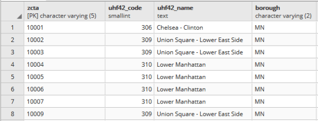
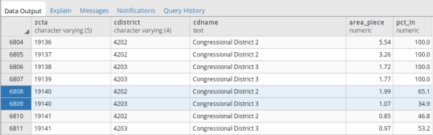
Portion of the ZCTA to UHF relational table.
In my first run through I simply tried to join the tables together using the 5-digit ZCTA to get the sum of households and aggregate incomes. I SUM the values for both and use GROUP BY to do the aggregation to UHF. In PostgreSQL pipe-forward slash: |/ is the operator for square root. I sum the squares for each ZCTA MOE and take the root of the total to get the UHF MOEs. I omit ZCTAs that have zero households so they’re not factored into the formulas:
SELECT z.uhf42_code, z.uhf42_name, z.borough,
    SUM(h.households) AS hholds,
    ROUND(|/(SUM(h.households_me^2))) AS hholds_me,
    SUM(a.agg_hhold_income) AS agghholds_inc,
    ROUND(|/(SUM(a.agg_hhold_income_me^2))) AS agghholds_inc_me
FROM zcta_uhf42 z, hsholds h, agg_income a
WHERE z.zcta=h.gid2 AND z.zcta=a.gid2 AND h.households !=0
GROUP BY z.uhf42_code, z.uhf42_name, z.borough
ORDER BY uhf42_code;
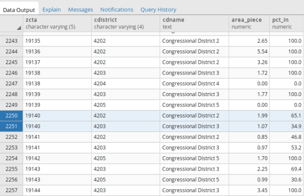
Portion of query result, households and income aggregated from ZCTA to UHF district.
Once that was working, I modified the statement to calculate mean income. Calculating the MOE for the mean looks pretty rough, but it’s simply because we have to repeat the calculation for the ratio over again within the formula. This could be avoided if we turned the above query into a temporary table, and then added two columns and populated them with the formulas in an UPDATE – SET statement. Instead I decided to do everything in one go, and just spent time fiddling around to make sure I got all the parentheses in the right place. Once I managed that, I added the ROUND function to each calculation:
SELECT z.uhf42_code, z.uhf42_name, z.borough,
    SUM(h.households) AS hholds,
    ROUND(|/(SUM(h.households_me^2))) AS hholds_me,
    SUM(a.agg_hhold_income) AS agghholds_inc,
    ROUND(|/(SUM(a.agg_hhold_income_me^2))) AS agghholds_inc_me,
    ROUND(SUM(a.agg_hhold_income) / SUM(h.households)) AS hhold_mean_income,
    ROUND((|/ (SUM(a.agg_hhold_income_me^2) + ((SUM(a.agg_hhold_income)/SUM(h.households))^2 * SUM(h.households_me^2)))) / SUM(h.households)) AS hhold_meaninc_me
FROM zcta_uhf42 z, hsholds h, agg_income a
WHERE z.zcta=h.gid2 AND z.zcta=a.gid2 AND h.households !=0
GROUP BY z.uhf42_code, z.uhf42_name, z.borough
ORDER BY uhf42_code;
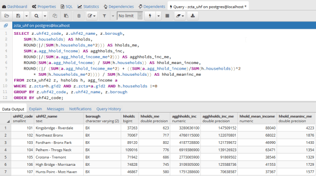
Query in pgAdmin and portion of result for calculating mean household income
I chose a couple examples where a UHF had only one ZCTA, and another that had two, and tested them in the Cornell ACS calculator to insure the results were correct. Once I got it right, I added:
CREATE VIEW household_sums AS
To the top of the statement and executed again to save it as a view. Mission accomplished! To make doubly sure that the values were correct, I connected my db to QGIS and joined this view to a UHF shapefile to visually verify that the results made sense (could also have imported the shapefile into the DB as a spatial table and incorporated it into the query).
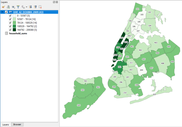
Mean household income by UHF neighborhood in QGIS
Conclusion
While it would be preferable to have a median, calculating a new mean for an aggregated area is a fair alternative, if you simply need some summary value for the variable and don’t have the time to spend doing statistical interpolation. Besides income, the Census Bureau also publishes aggregate tables for other variables like: travel time to work, hours worked, number of vehicles, rooms, rent, home value, and various subsets of income (earnings, wages or salary, interest and dividends, social security, public assistance, etc) that makes it possible to calculate new means for aggregated areas. Just make sure you use the appropriate denominator, whether it’s total population, households, owner or renter occupied housing units, etc.


You must be logged in to post a comment.