
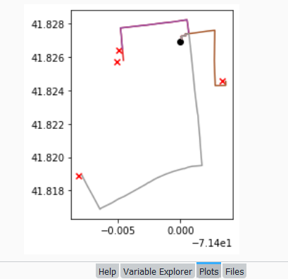
In this post I’ll demonstrate one method for assigning random colors to features on a Folium map, with specific consideration for plotting features from a geopandas geodataframe. I’m picking up where I left off in my previous post, where we plotted routes from a file of origins and destinations using the OpenRouteService. I wrote a regular Python script where I made a simple plot of the points and lines using geopanda’s plot, but in a Jupyter Notebook version I went a step further and used Folium to plot the features on the OpenStreetMap.
Folium is a Python port of Leaflet, a popular javascript library for making basic interactive web maps. I’m not going to cover the basics in this post, so for starters you can view Folium’s documentation: there’s a basic getting started tutorial, and a more detailed user guide. Geopanda’s documentation includes Folium examples that illustrate how you can work with the two packages in tandem.
One important concept to grasp, is that many of the basic examples assume you are working with latitude and longitude coordinates that are either hard-coded as variables, stored in lists, or stored in dedicated columns in a dataframe as attributes. But if you are working with actual geometry stored in a geodataframe, to display features you need to use the folium.GeoJson function instead. For example, this tutorial illustrates how to render points stored in a dedicated geometry column, and not as coordinates stored as numeric attributes in separate columns.
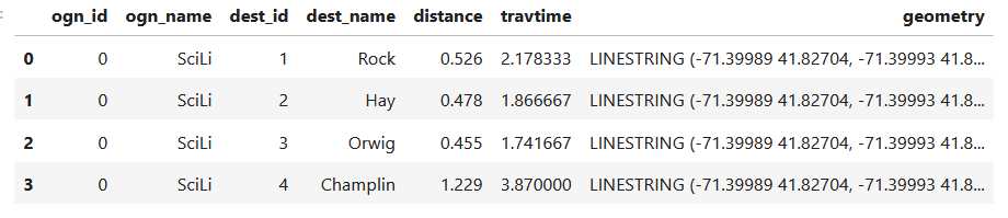
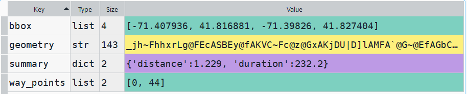
In my example, I have the following geodataframe, where each record is a route with linear geometry, with a sequential integer as the index value:
All I wanted to do was assign random colors to each line to depict them differently on the map – and I could not find a straightforward way to do that! In odd contrast, making a choropleth map (i.e. values shaded by quantity) seems easy. I found a couple posts on stack exchange, here and here, that demonstrated how to create and assign colors by randomly creating hexadecimal color strings. Another post illustrated how to assign specific non-random colors, and this thorough blog post walked through assigning colors to categorical data (where each category gets a distinct color).
I pooled aspects of the last two solutions together to come up with the following:
# Get colors for lines
gdfcount=len(gdf) # number of routes
colors=['red','green','blue','gray','purple','brown']
clist=[] # list of colors, one per route
c=0
for i in range(gdfcount):
clist.append(colors[c])
c=c+1
if c>len(colors)-1:
c=0 # if we run out of colors, start over
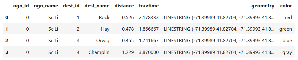
color_series = pd.Series(clist,name='color') # create series in order to...
gdf_c=pd.merge(gdf, color_series, left_index=True,right_index=True) # join to routes on seq index #
gdf_c
I get the number of features in my geodataframe, and create a list with a set number of colors. I iterate through my colors list, generating a new list with one color for each record in my frame. If I cycle through all the colors, I reset a counter and cycle through again from the beginning. When finished, I turn the list into a pandas series, which generates a sequential integer index paired with the color. Then I merge the series with my geodataframe (called gdf) using the sequential index, so the color is now part of each record:
Then I can create the map. When creating a Folium map you need to provide a location on which the map will be centered. I used Geopanda’s total_bounds method to get the bounding box of my features, which returns a list of coordinates: min X, min Y, max X, max Y. I sum the appropriate coordinates for X and Y and divide each by two, which gives me the coordinate pair for the center of the bounding box.
bnds=gdf.total_bounds
clong=(bnds[0]+bnds[2])/2
clat=(bnds[1]+bnds[3])/2
Next, I generate the map using those coordinates (the name of the map object in the example is “m”). I create a popup menu first, specifying which fields from the geodataframe to display when you click on a line. Then I add the actual geodataframe to the map, applying a style_function parameter to apply the colors and popup to each feature. The lambda business is necessary here, apparently when you’re applying styles that differ for each feature you have to iterate over the features. I guess this is the norm when you’re styling a GeoJSON file (but is at odds with how you would normally operate in a dataframe or GIS environment).
m = folium.Map(location=[clat,clong], tiles="OpenStreetMap")
popup = folium.GeoJsonPopup(
    fields=["ogn_name", "dest_name","distance","travtime"],
    localize=True,
    labels=True)
folium.GeoJson(gdf_c,style_function=lambda x: {'color':x['properties']['color']},popup=popup).add_to(m)
Once the lines are added to the map, we can continue to add additional features. I use folium.GeoJson twice more to plot my origin and destination points. It took me quite a bit of searching around to get the syntax right, so I could change the icon and color. This tutorial helped me identify the possibilities, but again the basic iteration examples don’t work if you’re using GeoJSON or geometry in a geodataframe. If you’re assigning several different colors you have to apply lambda, as in this example in the Folium docs. In my case I just wanted to change the default icon and color and apply them uniformly to all symbols, so I didn’t need to iterate. Once you’ve added everything to the map, you can finally display it!
folium.GeoJson(ogdf,marker=folium.Marker(icon=folium.Icon(icon='home',color='black'))).add_to(m)
folium.GeoJson(dgdf,marker=folium.Marker(icon=folium.Icon(icon='star',color='lightgray'))).add_to(m)
m.fit_bounds(m.get_bounds()) # zoom to bounding box
m
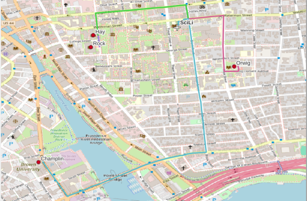
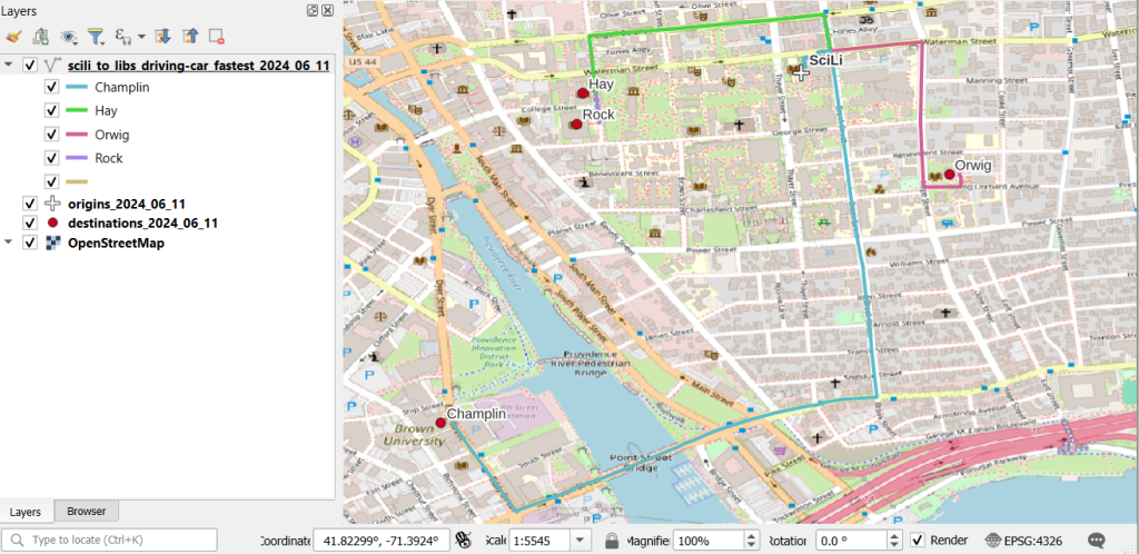
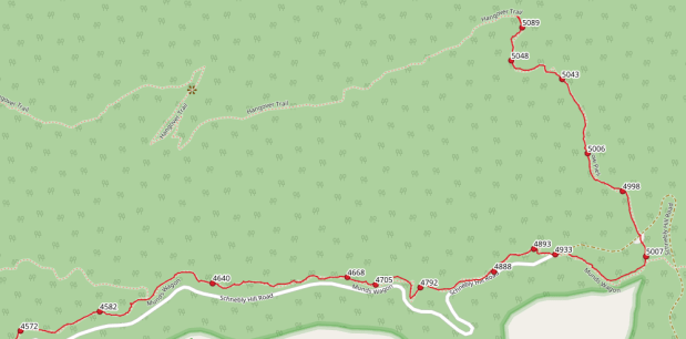
A static screenshot of the result follows, as I can’t embed Folium maps into my WordPress site. Everything works perfectly when using the notebook locally, but GitHub won’t display the map either, even if the Notebook is saved as a trusted source. If you open the notebook in the nbviewer, it renders just fine (scroll to the bottom of the notebook to see the map and interact).

Undoubtedly there are other options for achieving this same result. I saw examples where people had embedded all the styles they needed within a dedicated dataframe column as code and applied them, or wrote a function for applying the styles. I have rarely worked with javascript or coded my own web maps, so I expect there may be aspects of doings things in that world that were ported over to Folium that aren’t intuitive to me. But not being able to readily apply a random color scheme is bizarre, and is a big shortcoming of the module.
I’d certainly benefit from a more formal introduction to Folium / Leaflet, as scattered blog posts and stack exchange solutions can only take you so far. But here’s hoping that this post has added some useful scraps to your knowledge!


You must be logged in to post a comment.