The OpenStreetMap (OSM) can be a good source of geospatial data for all sorts of features, particularly for countries where the government doesn’t provide publicly accessible GIS data, and for features that most governments don’t publish data for. In this post I’ll demonstrate how to download a specific feature set for a relatively small area using QGIS 3.x. Instead of simply adding OSM as a web service base map we’ll extract features from OSM to create vector layers.
In the past I followed some straightforward instructions for doing this in QGIS 2.x, but of course with the movement to 3.x the core OSM plugin I previously used is no longer included, and no updated version was released. It’s a miracle that anyone can figure out what’s going on between one version of QGIS and the next. Fortunately, there’s another plugin called QuickOSM that’s quite good, and works fine with 3.x.
Use QuickOSM to Extract Features
Let’s say that we want to create a layer of churches for the city Merida in Mexico. First we launch QGIS, go to the Plugins menu, and choose Manage and Install plugins. Select plugins that are not installed, do a search for QuickOSM, select it, and install it. This adds a couple buttons to the plugins toolbar and a new sub-menu under the Vector menu called Quick OSM.
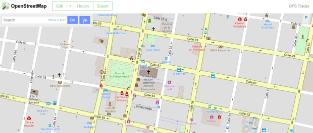
Next, we add a layer to serve as a frame of reference. We’re going to use the extent of the QGIS window to grab OSM features that fall within that area. We could download some vector files from GADM or Natural Earth; GADM provides several layers of administrative divisions which can be useful for locating and delineating our area. Or we can add a web service like OSM and simply zoom in to our area of interest. Adjust the zoom so that the entire city of Merida fits within the window.

OSM XYZ Tiles in QGIS – Zoomed into Merida
Now we can launch the Quick OSM tool. The default tab is Quick query, which allows us to select features directly from an OSM server (you need to be connected to the internet to do this). OSM data is stored in an XML format, so to extract the data we want we’ll need to specify the correct elements and tags. Ample documentation for all the map features is available. In our example, churches are referred to as places of worship and are classified as an amenity. So we choose amenity as the key and place_of_worship as the value. The drop down box allows us to search for features in or around a place, but as discussed in my previous post place names can be ambiguous. Choose the option for canvas extent, and that will capture any churches in our map window. Hit the advanced drop down arrow, and you have the option to select specific types of geometry (keep them all). Hit the run query button to execute.
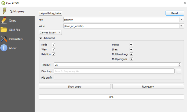
Quick OSM Interface
We’ll see there are two results: one for places of worship that are points, and another for polygons. If you right click on one of these layers and open the attribute table, you’ll see a number of tags that have been extracted and saved as columns, such as the name, religion, and denomination. The Quick query tools pulls a series of pre-selected attributes that are appropriate for the type of feature.

The data is saved temporarily in memory, so to keep it you need to save each as a shapefile or geopackage (right click, Export, Save Features As). But before we do that – why do have two separate layers to begin with? In some cases the OSM has the full shape of the building saved as a polygon, while in other cases the church is saved as a point feature, with a cross or other religious symbol appropriate for the type of worship space. It simply depends on the level of detail that was available when the feature was added.
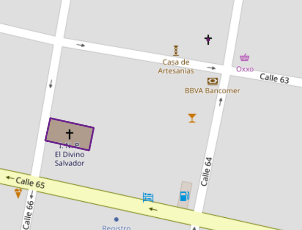
Church as polygon (lower left-hand corner) and as point (upper right-hand corner)
If we needed a single unified layer we would need to merge the two, but this process can be a pain. Using the vector menu you can convert the polygons to points using the centroid tool, and then use the merge tool to combine the two point layers. This is problematic as the number of fields in each file is different, and because the centroid tool changes the data type of the polygon’s id number to a type that doesn’t match the points. I think the easiest solution is to load both layers into a Spatialite database and create a unified layer in the DB.
Use SpatiaLite to Create a Single Point Layer
To do that, right click on the SpatiaLite option in the Browser Panel, choose Create Database, and name it (merida_churches). Then select the church point file, right click, export, save features as. Choose SpatiaLite as the format, for the file select the database we just created, and for layer name call it church_points. The default CRS (used by OSM) is WGS 84. Hit OK. Then repeat the steps for the polygons, creating a layer called church_polygons in that same database.
Once the features are database layers, we can write a SQL script (see below) where you create one table that has columns that you want to capture from both tables. You load the data from each of the tables into the unified one, and as you are loading the polygons you convert their geometry to points. The brackets around the names like [addr:full] allows you to overcome the illegal character designation in the original files (you shouldn’t use colons in db column names). I like to manually insert a date so to remember when I downloaded the feature set.
BEGIN;

CREATE TABLE all_churches (
full_id TEXT NOT NULL PRIMARY KEY,
osm_id INTEGER NOT NULL,
osm_type TEXT,
name TEXT,
religion TEXT,
denomination TEXT,
addr_housenumber TEXT,
addr_street TEXT,
addr_city TEXT,
addr_full TEXT,
download_date TEXT);

SELECT AddGeometryColumn('all_churches','geom',4326,'POINT','XY');

INSERT INTO all_churches
SELECT full_id, osm_id, osm_type, name, religion, denomination,
[addr:housenumber], [addr:street], [addr:city], [addr:full],
'02/11/2019', ST_CENTROID(geometry)
FROM church_polygons;

INSERT INTO all_churches
SELECT full_id, osm_id, osm_type, name, religion, denomination,
[addr:housenumber], [addr:street], [addr:city], [addr:full],
'02/11/2019', geometry
FROM church_points;

SELECT CreateSpatialIndex('all_churches', 'geom');

COMMIT;
Unfortunately the QGIS DB Browser does not allow you to run SQL transactions / scripts. You can paste the entire script into the window, highlight the first statement (CREATE TABLE), execute it, then highlight the next one (SELECT AddGeometryColumn), execute it, etc. Alternatively if you use the Spatialite CLI or GUI, you can save your script in a file, load it, and execute it in one go.

When finished we hit the refresh button and can see the new all_churches layer in the DB. We can preview the table and geometry and add it to the QGIS map window. If you prefer to work with a shapefile or geopackage you can always export it out of the db.
Other Options
The QuickOSM tool has a few other handy features. Under the Quick query tool is a plain old Query tool, which shows you the actual query being passed to the server. If you’re familiar with the map features and XML structure of OSM you can modify this query directly. Under the Query tool is the OSM File tool. Instead of grabbing features from the server, you can download an OSM pbf file (Geofabrik provides data for each country) and use this tool to load data from that file. It loads all features from the file for the geometries you choose, so the process can take awhile. You’ll want to load the data into a temporary file instead of saving in memory, to avoid a crash.
