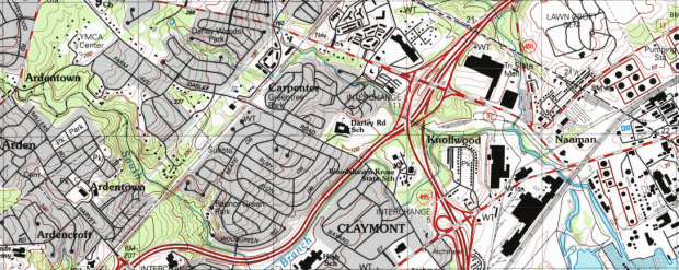
I was working with a graduate student last month who was looking for contour lines for specific towns within the US, for large-scale (small area) mapping and analysis. They were specifically interested in elevation for landfills, and some of the contour data they found didn’t map these as they aren’t natural features. We looked at current USGS topographic maps, and they do indeed map contours for landfills. But the topo maps are raster images, and they wanted vectors. Is it possible to access the underlying GIS data that was used to create the topo maps?
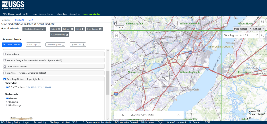
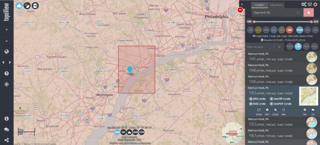
Indeed, it is! Option 1 is to use the National Map Download app. Search for a place name to zoom into your area of interest. Use the Show Map Index dropdown menu to draw the quad boundaries for the topo scale you’re interested in on the map; the 7.5 minute / 1:24,000 series is the USGS topo scale that most people are familiar with. Adjust the zoom so your area of interest fits within the map window; that way when you search in the Datasets tab on the left, the default search looks within this map extent.
Next, choose the specific data product you’re interested in. Here’s a list and description of all the National Map Datasets. For example, if you just wanted contour lines, you can select that under Small-scale Datasets. Note that raster imagery and data that’s used to derive the vectors is also available for download. If you want all the vector features that appear on a particular topo map, check the Topo Map Data and Topo Stylesheet option. Once you check a product, you can choose a file format for the data. Given the size of these datasets, the FileGDB option is probably best.
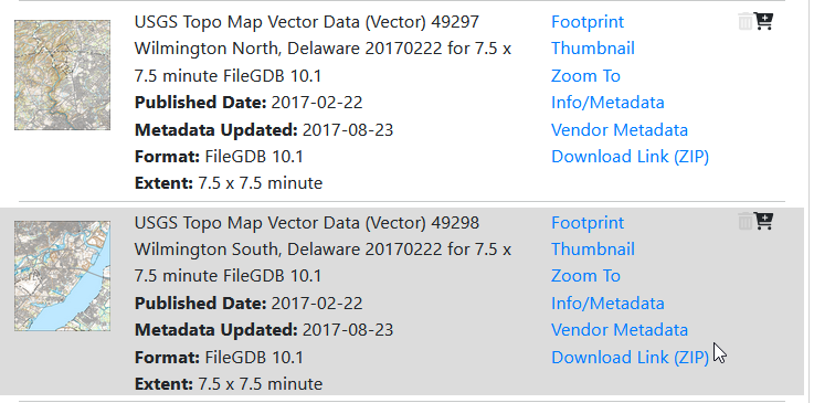
Then, click the blue Search Products button. That flips you to the Products tab, and displays data available within the extent of the map view. If you chose Topo Map Data and Topo Stylesheet, the results will be maps of individual quads. You can add a bunch of maps to your shopping cart by clicking on the little cart icon, or download one immediately by clicking the Download Link (ZIP).
Option 2 for downloading data: skip the map interface and use the Stage Products Directory. This no frills option is good if you know exactly which products you’re looking for. For example, you can drill down through TopoMapVector, then by state, and then data format to get to the same files you would have downloaded via option 1. You would need to know the name of the quad that encompasses the area you want; consult an index to figure it out.
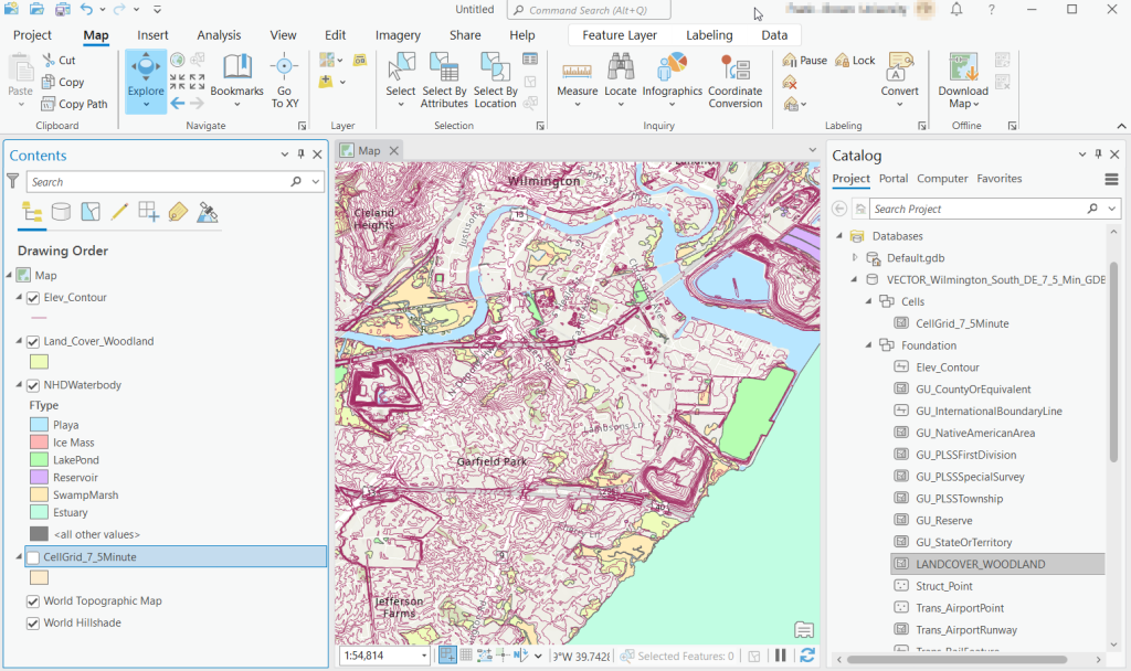
Once you download and unzip the file, you can launch your desktop GIS package to connect to the database and view the contents. In ArcGIS Pro, use the Catalog Pane, select the Databases option, right click, and Add Database. Browse to the location where you unzipped it, and select it. Then hit the dropdown for the newly added database and browse the contents, which are divided into schemas or groups. Foundation and Hydrography contain most of the features. GazVector has place name labels not captured in other features, and Cells contains outlines of the quad grid cells. Drag them into the Map Pane to view them.
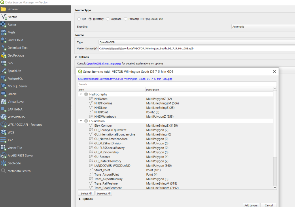
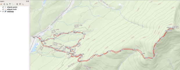
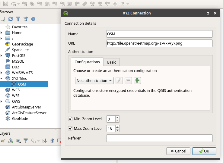
QGIS users can use the Data Source Manager. With the Vector option selected, change the Source Type from File to Directory, and in the Type dropdown choose OpenFileGDB. Then hit the dots button to browse your file system and select the database folder. Click Add, and you’ll be prompted to choose layers and tables to add to a project. You’ll see the same schema organization described previously, and you can use the CTRL and / or Shift keys to select what you want. Add the Layers, hit OK, and close the Manager.
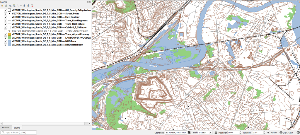
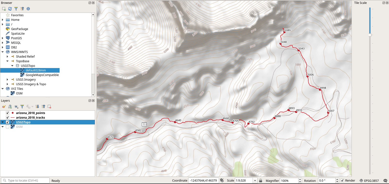
From there, it takes some artful manipulation of the overlays, color schemes, and labels to clearly symbolize the features. Both ArcGIS and QGIS have default symbol styles for topographic features that you can choose from. Apparently there’s a stylesheet packaged with the data, but I haven’t dug in enough yet to find and apply it. The attributes for the features seem fairly rich; the table includes columns that indicate the original data source for each feature, dates when records were added or updated, and a number of identifiers, labels, and categories. Some of the features, like bodies of water and county boundaries, extend beyond the quad cell for the map, as the USGS opted to keep whole features rather than clipping them. If the area you’re interested in happens to fall across two maps, you can download the topo map vector data for both quads, and use the Merge tool to combine them. The default CRS is un-projected NAD83 (EPSG 4269). You’ll probably want to reproject to a state plane or UTM zone that’s appropriate for your area. These post that describe styling and labeling contour lines in QGIS and ArcGIS Pro are helpful. Happy mapping!


You must be logged in to post a comment.