HIFLD Open, a key repository for accessing US GIS datasets on infrastructure, is shutting down on August 26, 2025. This is a revision from a previous announcement, which said that it would be live until at least Sept 30. The portal provided national layers for schools, power lines, flood plains, and more from one convenient location. DHS provides no sensible explanation for dismantling it, other than saying that hosting the site is no longer a priority for their mission (here’s a copy of an official announcement). In other words, “Public domain data for community preparedness, resiliency, research, and more” is no longer a DHS priority.
The 300 plus datasets in Open HIFLD are largely created and hosted by other agencies, and Open HIFLD was aggregating different feeds into one portal. So, much of the data will still be accessible from the original sources. It will just be harder to find.
DHS has published a crosswalk with links to alternative portals and the source feeds for each dataset, so you can access most of the data once Open HIFLD goes offline. I’ve saved a copy here, in case it also disappears. Most of these sources use ESRI REST APIs. Using ArcGIS Online or Pro, and even QGIS (for example), you can connect to these feeds, get a listing in your contents pane, and drag and drop layers into a project (many of the layers are also available via ArcGIS Online or the Living Atlas if you’re using Arc). Once you’ve added a layer to a project, you can export and save local copies.
Adding ArcGIS Rest Server for US Army Corps of Engineers Data in QGIS
If you want to download copies directly from Open HIFLD before it vanishes on Aug 26, I’ve created this spreadsheet with direct links to download pages, and to metadata records when available (some datasets don’t have metadata, and the links will bring you to an empty placeholder). Some datasets have multiple layers, and you’ll need to click on each one in a list to get to it’s download page. In some cases there won’t be a direct download link, and you’ll need to go to the source (a useful exercise, as you’ll need to remember where it is in the future). Alternatively, you can connect to the REST server (before Aug 26, 2025) in QGIS or ArcGIS, drag and drop the layers you want, and then export:
I’m coordinating with the Data Rescue Project, and we’re working on downloading copies of everything on Open HIFLD and hosting it elsewhere. I’ll provide an update once this work is complete. Even though most of these datasets will still be available from the original sources, better safe than sorry. There’s no telling what could disappear tomorrow.
The secure HIFLD site for registered users will remain available, but many of the open layers aren’t being migrated there (see the crosswalk for details). The secure site is available to DHS partners, and there are restrictions on who can get an account. It’s not exactly clear what they are, but it seems unlikely that most Open users will be eligible: “These instructions [for accessing a secure account] are for non-DHS users who support a homeland security or homeland defense mission AND whose role requires access to the Geospatial Information Infrastructure (GII) and/or any geospatial dashboards, data, or tools housed on the GII…“
Let’s say you have different sets of points, and each set represents a distinct category of features. Maybe villages where residents speak different languages, or historical events that occurred during different epochs. Beyond plotting and symbolizing the points, perhaps you would like to create areas for each set that represent generalized territory, and you’d like to see how these areas correspond. I’ll demonstrate a few approaches for achieving this, using convex hulls, attribute table calculations, and geoprocessing tools like intersection and union. A convex hull is a minimum bounding polygon, where an area is drawn around all points in a set, where the outermost points serve as vertices for creating boundaries.
I’ll use QGIS for this example, but will mention the corresponding tools in ArcGIS Pro at the end. In QGIS we’ll use the tools that are located within the Processing Toolbox (gear icon on the toolbar). Unlike the shortcut tools under the Vector menu, these tools provide more options and allow us to process multiple files at once.
Steps in QGIS
First, we need either distinct point files for each set of features, or a single file with a categorical variable that distinctly identifies different sets of features. For this example I’ll use three distinct files that I’ve generated using phony sample data. The points are in a projected coordinate system (important!) that’s appropriate for the area I’m mapping.
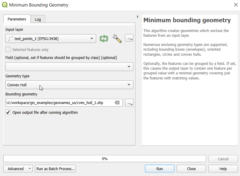
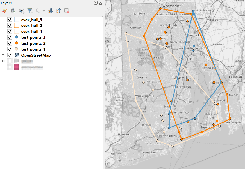
In the QGIS Processing Toolbox, we select the Minimum Bounding Geometry (MBG) tool, and under the Geometry Type specify that we want to create a convex hull. I ran this tool for each file, creating three convex hull files (alternatively, if you had one file with distinct categories, you could use the Field option to generate separate hulls for each category). I’ve symbolized the output below, making the fill hollow and assigning an outline that matches the color of the points. This gives you a good sense for the coverage areas for the points, and how they overlap.
Before running additional tools to explicitly measure overlap, we need to modify the attribute tables of the convex hulls, so we’ll have useful attributes to carry over. The MBG tool creates a new layer with an ID number, area, and perimeter. The ID is set to zero for each hull file, but we should change it to distinctly represent the file / category. With the attribute table open, we can go into an edit mode and type in a new integer value; in this case I’m assigning 1, 2, and 3 to each of the test layers. Alternatively, you could add a new field and assign it a meaningful category value.
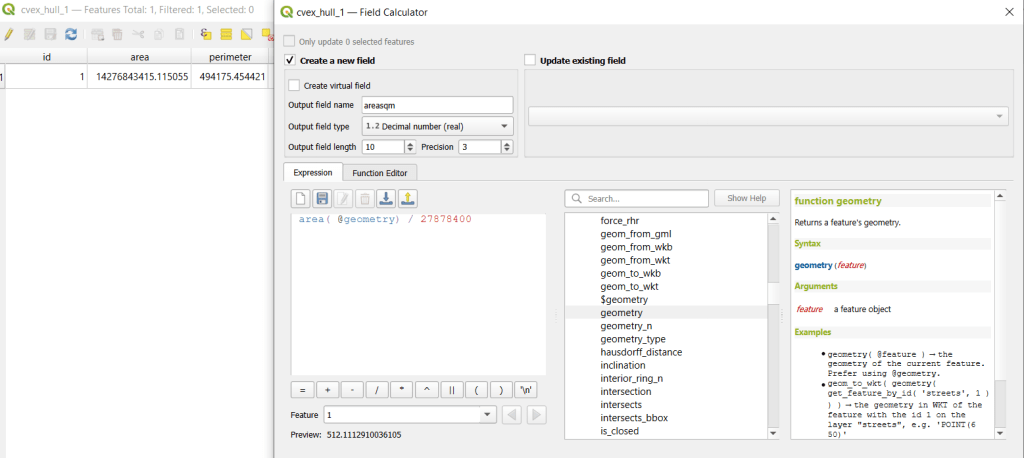
The units for area and perimeter match the units used by the map projection of the layer, which is why we want to use a projected coordinate system that uses meters or feet, and not a geographic one (like WGS 84 or NAD 83) that uses degrees. I’m using a state plane system, so the area is in square feet. To convert this to square miles, within the attribute table view I use the Field Calculator to add a new decimal field, and divide the value of the area by 27,878,400 (the number of sq feet in a sq mile; for metric units in meters, we’d divide by 1,000,000 to get sq km). We calculate the area directly from the polygon geometry:
area( @geometry) / 27878400
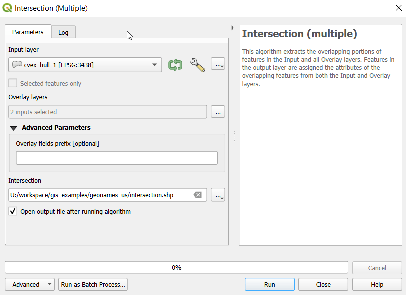
To generate the area of intersection, we go into the Processing tool box and run the Intersection (multiple) tool. The first convex hull is the input layer, while the overlay layers are the other two hull files (in the dialog box, we check the layers we want, and then use the arrow to navigate back to the tool to run it). The output is a new file with polygon(s) that cover the area where all three layers intersect. Its attribute table contains an ID, area, and perimeter field, and we can calculate a new area field in sq miles and see how it compares to the total areas. In my example, the area where all three territories intersect covers about 112 sq miles, while the areas for the individual territories are 512, 563, and 256 sq miles respectively.
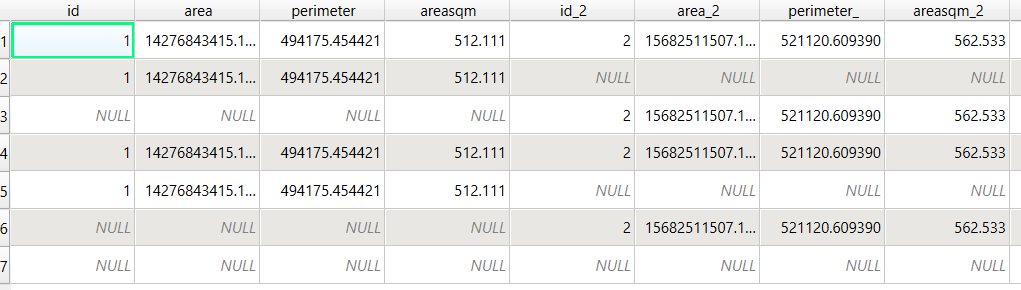
To identify distinct areas of overlap between the territories, we return to the Processing toolbox and run the Union (multiple) tool. The dialog is similar to the intersection tool, where the first hull is the union layer and the additional hulls are overlay layers. The output of this tool is a layer with distinct polygons where the hulls coincide. The attribute table for the union layer carries over the attributes from each of the three layers, with columns suffixed with underscores and sequential integers. So if a polygon consists of area covered by hulls 1 and 2, those attributes will be filled in, while the attributes of 3 will be null. As before, we can calculate an area in sq miles for the new polygons. In this case, we’d see that the area covered by hull 1 without any overlapping hulls is 240 sq miles, the largest of all territories.
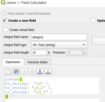
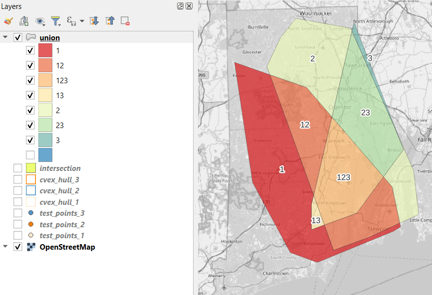
To explicitly categorize these areas, we can add a new field in the attribute table. This will be a text field, where we take the ID numbers, convert them to strings, and concatenate them. In the example above, IDs 1 and 2 would be concatenated to 12, and since the value for 3 is null, no text is appended. (Variation – if you created distinct text-based category fields instead of using the integer IDs, you could concatenate them directly without having to convert them to strings). Using the symbology tool, we can classify the data using these new categories, and can modify the color scheme to something appropriate for displaying the contributions from each area. So a polygon with category 1 includes areas covered by the first convex hull and no others, while category 12 includes areas where hulls 1 and 2 overlapped.
With the areas of the individual union pieces, we can compute the percentages of each territory that fall inside and outside various overlapping zones with the field calculator. For example, we can calculate the total area of the union file (which is NOT the sum of each hull, as there’s overlap between them), and then divide each feature by that total to get its percent total. The expression for doing this is below; the numerator has the name of the field that contains the area of each polygon in sq miles, while the denominator includes the calculation for the sum of all parts (alternatively you could use the QGIS Statistics tool to compute this, and hard code the total into the formula):
If the idea is to create areas of territory that the points exert influence on, you may want to add a buffer to each hull, to account for the fact that the outer points that form the boundaries will exert influence on both sides of the boundary. Use the Processing – Buffer tool. For the buffer distance, you can use an arbitrary value that makes sense for the circumstances. Or you can generate a relative value that represents a fraction of each convex hull’s area. The output of the buffer tool would then serve as the input to the intersection and union tools.
These examples focus on area. If the number of points that falls within the areas is important, you can use the Points in Polygon tool on each of the hulls to count points, and then do the same for the output of the intersection and union tools to get the different points counts for each set of polygons.
ArcGIS Pro Corollaries
Following the same steps above for QGIS, but with ArcGIS Pro:
In the red toolbox, the Minimum Boundary Geometry tool is used to create convex halls. It’s quite similar to the one in QGIS: specify the geometry type, and there is an option to Group (if you have one file with categories). If you leave the Add geometry characteristics box unchecked, it will still compute basic area and perimeter; the checkbox adds a bunch of additional fields.
Unlike QGIS, ArcGIS will not allow you to modify its OBJECTID field. To create a unique value for each hull, you will have to open the attribute table and use the Calculate tool to create a category field (integer or text). To ensure that you can carry it over, in ArcGIS you need to give this column a different name in each hull: cat1, cat2, cat3. Set the value at the bottom in the expression box.
You can use the calculate tool in the attribute table to generate an area column in sqft or sqkm, or use the Calculate Geometry Tool in the toolbox instead. The latter is actually simpler: create a new column, and choose Area and the output units.
The Intersect tool will create the intersection, and functions similarly to QGIS.
The Union tool creates the union, and also functions similarly.
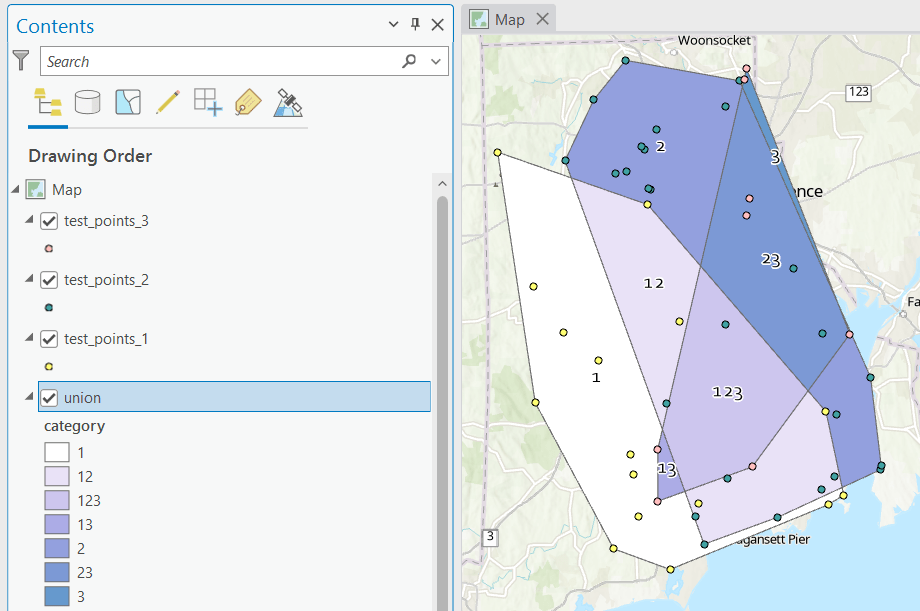
Creating the category field in the union file is a bit more complicated, as ArcGIS assigns values of 0 instead of NULL for non-overlapping polygons. In the Calculate window, with the input file as Union and the field as category, change the Expression type to Arcade (ESRI’s scripting language). First, run an expression to concatenate the categories and convert integers to strings (if necessary). Then, replace that expression with a second one that replace the zeros with nothing.
This is a basic approach, appropriate for certain use cases where you want to generate areas from points; particularly when different point sets have a well defined category, so there’s no question of how to group them. Also appropriate where you don’t have – or don’t want – hard boundaries between sets of points and want to see areas of overlap. More sophisticated methods exist for separating points into clusters based on density, distance, and similar attributes, such as K-Means and DB Scan. You can generate non-overlapping territories for individual points using Thiessen / Voronoi polygons, and for points with a sufficiently high density, you can generate rasters with kernel tools.
I was working with a graduate student last month who was looking for contour lines for specific towns within the US, for large-scale (small area) mapping and analysis. They were specifically interested in elevation for landfills, and some of the contour data they found didn’t map these as they aren’t natural features. We looked at current USGS topographic maps, and they do indeed map contours for landfills. But the topo maps are raster images, and they wanted vectors. Is it possible to access the underlying GIS data that was used to create the topo maps?
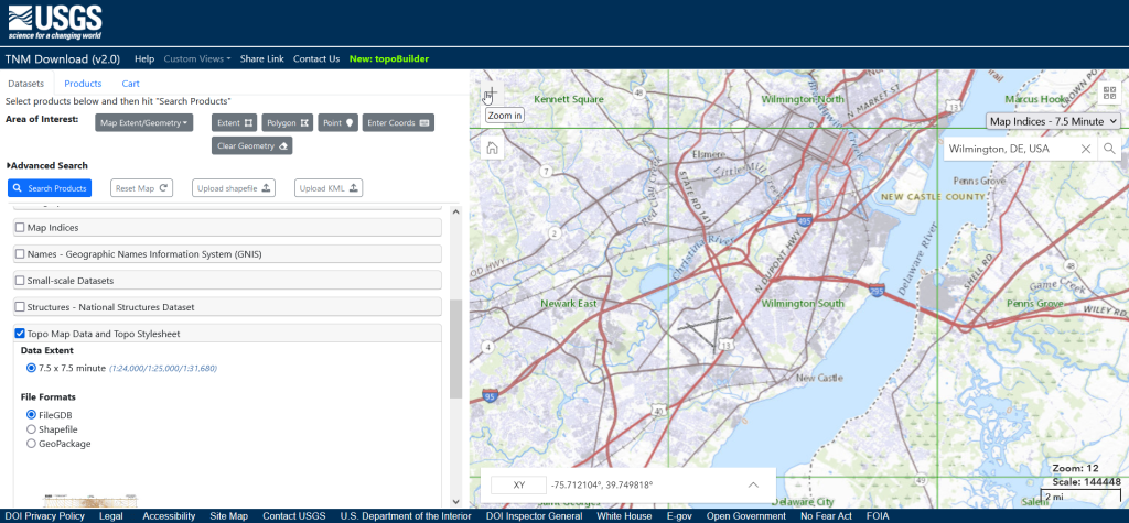
Indeed, it is! Option 1 is to use the National Map Download app. Search for a place name to zoom into your area of interest. Use the Show Map Index dropdown menu to draw the quad boundaries for the topo scale you’re interested in on the map; the 7.5 minute / 1:24,000 series is the USGS topo scale that most people are familiar with. Adjust the zoom so your area of interest fits within the map window; that way when you search in the Datasets tab on the left, the default search looks within this map extent.
Next, choose the specific data product you’re interested in. Here’s a list and description of all the National Map Datasets. For example, if you just wanted contour lines, you can select that under Small-scaleDatasets. Note that raster imagery and data that’s used to derive the vectors is also available for download. If you want all the vector features that appear on a particular topo map, check the Topo Map Data and Topo Stylesheet option. Once you check a product, you can choose a file format for the data. Given the size of these datasets, the FileGDB option is probably best.
The National Map Download Interface, Showing the Datasets Tab for Selecting and Searching
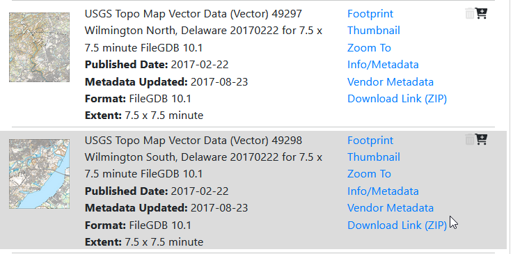
Then, click the blue Search Products button. That flips you to the Products tab, and displays data available within the extent of the map view. If you chose Topo Map Data and Topo Stylesheet, the results will be maps of individual quads. You can add a bunch of maps to your shopping cart by clicking on the little cart icon, or download one immediately by clicking the Download Link (ZIP).
On the Product Tab, click Download Link (ZIP) to get data for a specific map
Option 2 for downloading data: skip the map interface and use the Stage Products Directory. This no frills option is good if you know exactly which products you’re looking for. For example, you can drill down through TopoMapVector, then by state, and then data format to get to the same files you would have downloaded via option 1. You would need to know the name of the quad that encompasses the area you want; consult an index to figure it out.
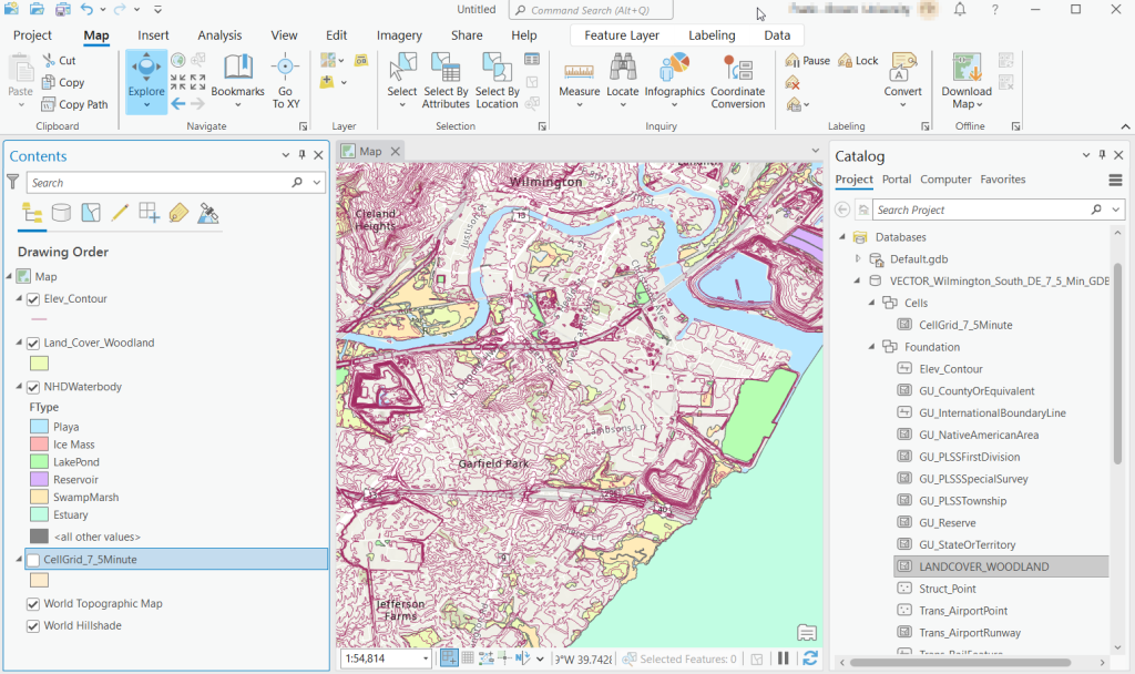
Once you download and unzip the file, you can launch your desktop GIS package to connect to the database and view the contents. In ArcGIS Pro, use the Catalog Pane, select the Databases option, right click, and Add Database. Browse to the location where you unzipped it, and select it. Then hit the dropdown for the newly added database and browse the contents, which are divided into schemas or groups. Foundation and Hydrography contain most of the features. GazVector has place name labels not captured in other features, and Cells contains outlines of the quad grid cells. Drag them into the Map Pane to view them.
USGS Topo Map Vector Data in ArcGIS Pro
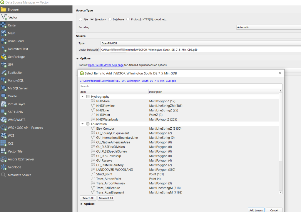
QGIS users can use the Data Source Manager. With the Vector option selected, change the Source Type from File to Directory, and in the Type dropdown choose OpenFileGDB. Then hit the dots button to browse your file system and select the database folder. Click Add, and you’ll be prompted to choose layers and tables to add to a project. You’ll see the same schema organization described previously, and you can use the CTRL and / or Shift keys to select what you want. Add the Layers, hit OK, and close the Manager.
Adding File Geodatabase Features in the QGIS Data Source Manager
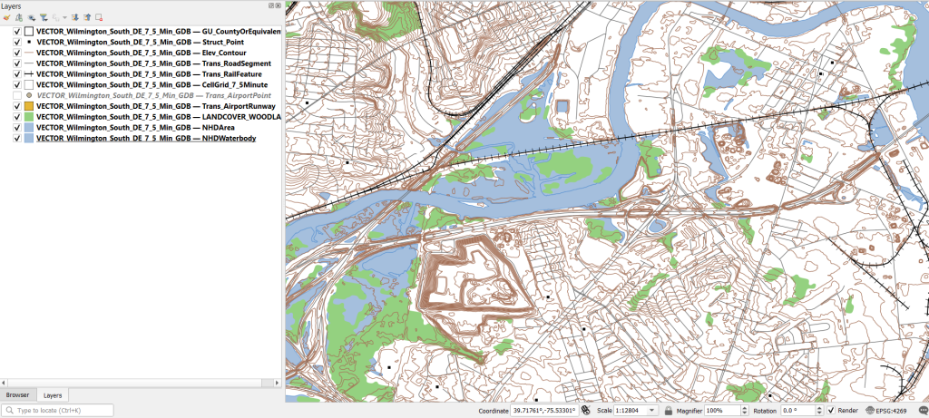
From there, it takes some artful manipulation of the overlays, color schemes, and labels to clearly symbolize the features. Both ArcGIS and QGIS have default symbol styles for topographic features that you can choose from. Apparently there’s a stylesheet packaged with the data, but I haven’t dug in enough yet to find and apply it. The attributes for the features seem fairly rich; the table includes columns that indicate the original data source for each feature, dates when records were added or updated, and a number of identifiers, labels, and categories. Some of the features, like bodies of water and county boundaries, extend beyond the quad cell for the map, as the USGS opted to keep whole features rather than clipping them. If the area you’re interested in happens to fall across two maps, you can download the topo map vector data for both quads, and use the Merge tool to combine them. The default CRS is un-projected NAD83 (EPSG 4269). You’ll probably want to reproject to a state plane or UTM zone that’s appropriate for your area. These post that describe styling and labeling contour lines in QGIS and ArcGIS Pro are helpful. Happy mapping!
It’s been a busy few months, but I have a few days to catch my breath now that it’s spring break and most people (except me) have gone away! One question that’s come up quite a bit this semester is how to associate raster data with coinciding vector data. I’ll summarize some approaches in this post using ArcGIS Pro and QGIS, to summarize raster values for polygons (zonal statistics) and to assign raster values to points (aka raster sampling).
Zonal Statistics: Summarize Rasters by Area
Imagine that you have quantitative values such as temperature or a vegetation index in a raster grid, and you want to use this data to calculate an average for counties or metro areas. The goal is to have a new attribute column in the vector layer that contains the summarized raster value, perhaps because you want to make thematic maps of that value, or you want to use it in conjunction with other variables to run spatial statistics, or you just want a plain and simple summary for given places.
The term zonal statistics is used to define any operation that calculates statistics on cell values of a raster within an area or zone defined by another dataset, either a raster or a vector. The ArcGIS Pro toolbox has a Zonal Statistics tool where the output is a new raster file with cells that are summarized by the input zones. That’s not desirable for the use case I’m presenting here; the better choice is the Zonal Statistics as Table tool. The output is a table containing the unique identifiers of the raster and vector, the summary stats you’ve generated (average, sum, min, max, etc), and a count of the number of cells used to generate the summary. You can join this resulting table back to the vector file using their common unique identifier in a table join.
In the example below, I’m using counties from the census TIGER files for southern New England as my Input Feature Zone, the AFFGEOID (Census ANSI / FIPS code) to identify the Zone Field, and a temperature grid for January 1, 2020 from PRISM as the Input Value Raster. I’m calculating the mean temperature for the counties on that day.
ArcGIS Pro Zonal Statistics as Table; Temperature Grid and Southern New England Counties
The output table consists of one record for each zone / county, with the count of the cells used to create the average, and the mean temperature (in degrees Celsius). This table can be joined back to the original vector feature (select the county feature in the Contents, right click, Joins and Relates – Join) to thematically map the average temp.
ArcGIS Pro Zonal Statistics; Table Output and Join to Show Average Temperature per County
In QGIS, this tool is simply called Zonal Statistics; search for it in the Processing toolbox. The vector with the zones is the Input layer, and the Raster layer is the grid with the values. By default the summary stats are the count, sum, and mean, but you can check the Statistics to calculate box to select others. Unlike ArcGIS, QGIS allows you to write output as a table or a new shapefile / geopackage, which carries along the feature geometry from the Input zones and adds the summaries, allowing you to skip the step of having to do a table join (if you opted to create a table, you could join it to the zones using the Joins tab under the Properties menu for the vector features).
QGIS Zonal Statistics
Extract Raster Values for Point Features
Zonal stats allows you to summarize raster data within a polygon. But what if you had point features, and wanted to assign each point the value of the raster cell that it falls within? In ArcGIS Pro, search the toolbox for the Extract Values to Points tool. You select your input points and raster, and a new point feature that will include the raster values. The default is to take the value for the cell that the point falls within, but there is an Interpolate option that will calculate the value from adjacent cells. The output point feature contains a new column called RASTERVALU. I created some phony point data and used it to generate the output below.
ArcGIS Pro Extract Values to Points (assign raster cell values to points)
In QGIS the name of this tool is Sample raster values, which you can find in the Processing toolbox. Input the points, choose a raster layer, and write the output to a new vector point file. Unlike ArcGIS, there isn’t an option for interpolation from surrounding cells; you simply get the value for the cell that the point falls within. If you needed to interpolate, you can go to the Plugins menu, enable the SAGA plugin, and in the Processing toolbox try the SAGA tool Raster Values to Points instead.
QGIS Sample Raster Values (assign raster cell values to points)
A variation on this theme would be to create and assign an average value around each point at a given distance, such as the average temperature within five miles. One way to achieve this would be to use the buffer tools in either ArcGIS or QGIS to create distinct buffers around each point at the specified distance. The buffer will automatically carry over all the attributes from the point features, including unique identifiers. Then you can run the zonal statistics tools against the buffer polygons and raster to compute the average, and if need be do a table join between the output table and the original point layer using their common identifier.
Wrap-up
In using any of these tools, it’s important to consider the resolution of the raster (i.e. the size of the grid cell):
1. Relative to the size of the zonal areas or number of points, and
2. In relation to the phenomena that you’re studying.
When larger grid cells or zonal areas are used for measurement, any phenomena becomes more generalized, and any variations within these large areas become masked. The temperature grid cells in this example had a resolution of 2.5 miles, which was suitable for creating county summaries. Summarizing data for census tracts at this resolution would be less ideal, as the tracts are much smaller than the cells, with the cell value characterizing a much larger area. This might be okay in the case of temperature, which tends not to vary considerably over a distance of a few miles. In contrast, averaging temperature data for states is not worthwhile, as states vary considerably in size and most are large enough that they contain multiple ecosystems and elevation levels.
The solutions I’ve described here are the desktop GIS solutions. You could also use either spatial SQL in a geodatabase or a spatial extension in a scripting language like Python or R to perform similar operations. In both cases a basic overlay and intersection statement is used, in conjunction with some grouping function for calculating summaries. I’ve been doing a lot more spatial Python work with geopandas these past few months – perhaps a topic for a subsequent post…
A couple years ago I wrote a post that demonstrated how to use the QuickOSM plugin for QGIS to easily extract features from the OpenStreetMap (OSM). The OSM is a great source for free and open GIS data, especially for types of features that are not captured in government sources, and for parts of the world that don’t possess a free or robust GIS data infrastructure. I’ve been using ArcGIS Pro more extensively in my new job and was wondering how I could do the same thing: query features from the OSM based on keys and values (denoting feature type) and geographic area and extract them as a vector layer. I’m looking for straightforward solutions that I could use for answering questions from students (so no command line tricks or database stuff). In this post I’ll cover three approaches for achieving this in ArcGIS Pro, with references to QGIS.
File Approach
The most straightforward method would be to export data directly from the main OSM page by zooming into an area and hitting the Export button. This is a pretty blunt approach, as you have to be zoomed in pretty close and you grab every possible feature in the view. The “native” file format of OSM is the osm / pbf format; .osm is an XML file while .pbf is a compressed binary version of the osm. QGIS is able to handle these files directly; you just add them as a vector layer. ArcGIS Pro cannot. You have to download and install a special Data Interoperability extension, which is an esoteric thing that’s not part of the standard package and requires a special license from your site license coordinator.
A better and more targeted approach is to download pre-created extracts that are provided by a number of organizations listed in the OSM wiki. I started with Geofabrik in Germany, as it was a source I recognized. They package OSM data by geographic area and feature type. On their main page they list files that contain all features for each of the continents. These are enormous files, and as such they are only provided in the osm pbf format as shapefiles can’t effectively handle data that size. Even if you downloaded the osm pbf files and added them to QGIS, the software will struggle to render something that big.
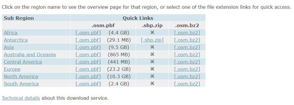
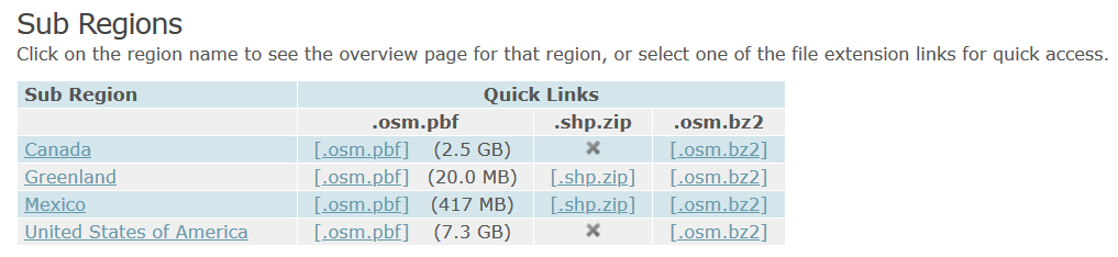
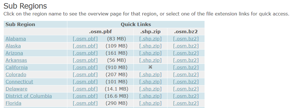
But all is not lost; Geofabrik and many other providers package data in a shapefile format for smaller areas, provided that the size and number of features is not too great. For instance, on Geofabrik’s download page if you click on North America you’re presented with country extracts for that continent (see images below). You can get shapefiles for Greenland and Mexico, but not Canada or the US as the files are still too big. Click on US, and you’re presented with files for each of the states. No luck for California (too big), but the rest of states are small enough that you can get shapefiles for all of them.
Default Geofrabrik OSM download page for continents. Click on a continent name…
…to access files for countries. Click on a country name…
…to access files for states / provinces / admin divisions
I downloaded and unzipped the file for Rhode Island. It contains a number of individual shapefiles classified by type of feature: buildings, land use, natural, places, places of worship (pofw), points of interest (pois), railways, roads, traffic, transport, water, and waterways. Many of the files appear twice: files with an “a” suffix represent polygons (areas) while files without that suffix are points or lines. Some OSM features are stored as polygons when such detail is available, while others are represented as points.
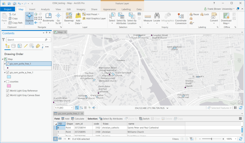
For example, if I add the two places of workship files to a map, for some features you have the outline of the actual building, while for most you simply have a point. After adding the layers to the map, you’ll probably want to use Select by Attribute to select the features you want based on OSM tags with keys and values, and Select by Location in conjunction with a separate boundary file to pull data out for a smaller area. The Geofabrik OSM attribute table is limited to basic attributes: an OSM ID, feature code and class, and name. It’s also likely that you’ll want to unify the point and polygon features of the same type into one layer, as they’re usually mutually exclusive. Use the Centroid (Polygon) tool in the toolbox to turn the polygons into points, and the Merge tool to meld the two point layers together. In QGIS the comparable tools under the Vector menu are Centroids and Merge Vector Layers. WGS 84 is the default CRS for the layers.
OSM Places of Worship. Some features are stored as points while others are polygons
Geofabrik is just one option. There are several others and they take different approaches for structuring their extracts. For example, BBBike.org organizes their layers by city for over 200 cities around the world, and they provide a number of additional formats beyond OSM PBF and shapefiles, such as Garmin GPS, GeoJSON, and CSV. They divide the data into fewer files, and if they don’t compile data for the area you’re interested in you can use a web-based tool to create a custom extract.
Plugin Approach
It would be nice to use a plugin, as that would allow you to specify a custom geographic area and retrieve just the specific features you want. QuickOSM works quite nicely for QGIS. Fortunately there is a good ArcGIS Pro solution called OSMquery. It works for both Pro and Desktop, tested for Pro 2.2 and Desktop 10.6. I’m using Pro 2.7 and the basic tool worked fine. It’s well documented, with good instructions for installation and use.
The plugin is written in Python and you add it as a tool to your ArcToolbox. Download the repo from the OSMquery GitHub as a ZIP file (click the green code button and choose Download ZIP). Save it in or near your ArcGIS project folders, and unzip it. In Pro, go into a project and open a Catalog Pane in the View ribbon. Right click on Toolbox to add a new one, and browse to the folder you unzipped to add the tool. There are two scripts in the box, a basic and an advanced version. The basic tool functioned without trouble for me. The advanced tool threw an error, probably some Python dependency issue (I didn’t investigate as the basic tool met my needs).
In the basic tool you choose the key and value for the features you want to extract; the dropdown menu is automatically populated with these options. For the geographic extent you can enter a place name, or you can use the extent of the current map window or of a layer in the project, or you can manually type in bounding box coordinates. Another nice option is you can transform the CRS of the extracted features from WGS 84 to another system, so it matches the CRS of layers in your existing project. Run the tool, and the features are extracted. If the features exist as both points and polygons, you get two separate files for each. If you choose, you can merge them together as described in the previous section; this is a bit tougher as the plugin approach yields a much wider selection of fields in the attribute table, and not all of the point and polygon attributes align. With the Merge tool in Pro you can select which attributes you want to hold on to, and common ones will be merged. QGIS is a bit messier in this regard, but in my earlier post I outlined a work-around using a spatial database.
The basic OSMquery tool in an ArcGIS Pro toolbox
Web Feature Service
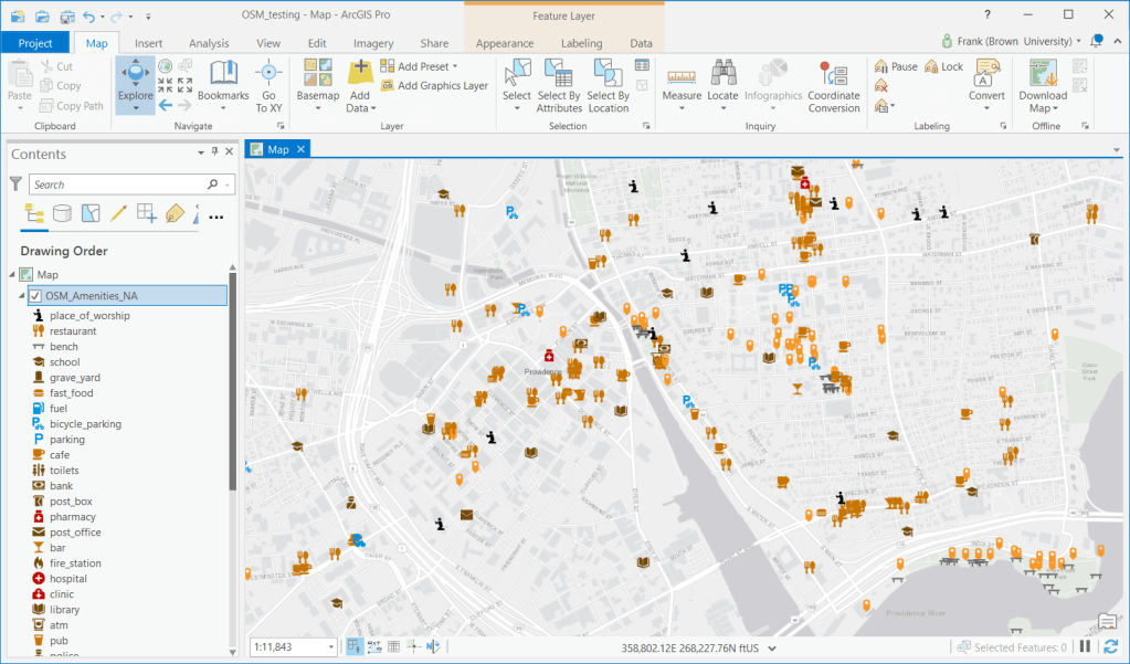
This initially seemed to be the most promising route, but it turned out to be a dud. Like QGIS, Pro allows you to add OSM as a tiled base map. But ESRI also offers OSM as a web feature service: by hitting Add Data on the Map ribbon and searching the Living Atlas for “OpenStreetMap” you can select from a number of OSM web feature services, organized by continent and feature type. Once you add them to a map, you can select and click on individual features to see their name and feature type. The big problem is that you are not allowed to extract features from these layers, which leaves you with an enormous and heterogeneous mix of features for an entire continent. You can interact with the features, selecting by attribute and location in reference to other spatial layers, but that’s about it.
OSM web feature service in ArcGIS Pro
In Summary
I would recommend taking the step of downloading the OSMquery plugin for ArcGIS Pro if you want to take a highly targeted approach to OSM feature extraction (for QGIS users, enable the QuickOSM plugin). This approach is also best if you can’t download a pre-existing extract for your area because it’s too large or has too many features, and if you want to access the fullest possible range of attribute values. Otherwise, you can simply download one of the pre-created extracts, and use your software to winnow it down to what you need (or if you do need everything, the file approach makes more sense). Since the file-based option includes fewer attributes, converting polygon features to points and merging them with the other point features is a bit simpler.
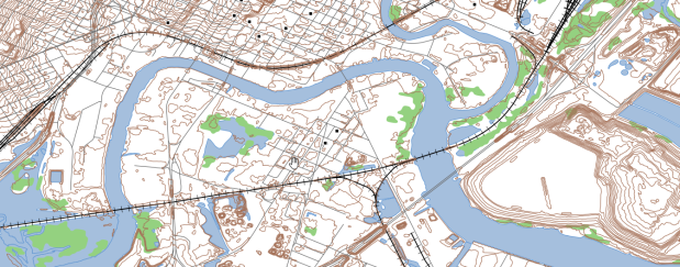
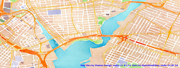
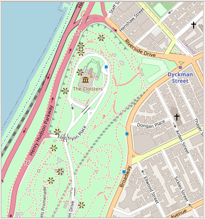
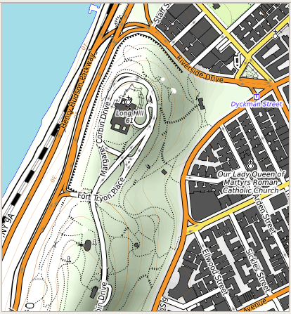
For this final post of 2020, I was looking back through recent projects for something interesting yet brief; I’ve been writing some encyclopedia-length posts lately and wanted to keep this one on the lighter side. In that vein, I’ve decided to share a short list of free web mapping services that I use as basemaps in QGIS (they’ll work in ArcGIS too). This has been on my mind as I’ve recently stumbled upon the OpenTopoMap, which is an alternate stylized version of the OpenStreetMap that looks pretty sharp.
Comparison of OpenStreetMap (left) and OpenTopoMap (right)
Select the appropriate web map service type in the browser panel (usually WMS / WMTS or XYZ Tiles), right click, and add new connection.
Give it a meaningful name, paste the appropriate URL into the URL box, click OK.
In the browser panel drill down to see the service, and for WMS / WMTS layers you can drill down further to see specific layers you can add.
Select the layer and drag it into the window, or select, right click, and add the layer to the project.
If the resolution looks off, right click on a blank area of the toolbar and check the Tile Scale Panel. Use this to adjust the zoom for the web map. If the scale bar is greyed out you’ll need to set the map window to the same CRS as the map service: select the layer in the panel, right click, and choose set CRS – set project CRS from layer.
Some web layers may render slowly if you’re zoomed out to the full extent, or even not at all if they contain many features or are super detailed. Conversely, some layers may not render if you’re zoomed too far in, as tiles may not be available at that resolution. Experiment!
If you’re an ArcGIS user see these concise instructions for adding various tile layers. This isn’t something that I’ve ever done, as ArcGIS already has a number of accessible basemaps that you can add.
In the list below, links for the service name take you to either the website version of the service, or to a list of additional layers that you can connect to. The URLs that follow are the actual connections to the service that you’ll use within your GIS package. If you use OSM, OTP, or Stamen in your maps, make sure to cite them (they use Creative Commons Licenses – follow links to their websites for details). The government sources are public domain, but you should still cite them anyway. Happy mapping, and happy holidays!
Current TIGER features:
https://tigerweb.geo.census.gov/arcgis/services/TIGERweb/tigerWMS_Current/MapServer/WMSServer

Current physical features:
https://tigerweb.geo.census.gov/arcgis/services/TIGERweb/tigerWMS_PhysicalFeatures/MapServer/WMSServer


You must be logged in to post a comment.