The U.S. Census Bureau’s County and ZIP Code Business Patterns (CBP and ZBP) datasets are generated annually from the Business Register, a large administrative database updated by several federal agencies which contains every business establishment in the U.S. with paid employees. Business establishments are defined as single physical locations where business is conducted or where services or industrial operations are performed. Establishments are assigned to industries, which are groups of businesses that produce similar products or provide similar services, using the North American Industrial Classification System (NAICS). The ZBP contains tables with total establishments, employment, and wages by ZIP and counts of business establishments by NAICS and ZIP. The CBP has these tables plus a few others for counties.

The 2017 Business Patterns was recently released, and there are a few important changes to the dataset over previous iterations. I’ll summarize what they are and how they impact data retrieval using the Census Bureau’s ZBP API. I unwittingly discovered these issues this week as I was trying to use a Python / Pandas notebook I’d written for extracting ZBP data and aggregating the USPS ZIP codes to Zip Code Tabulation Areas (ZCTAs), which are used for publishing decennial and ACS census data. Everything went smoothly when I tested the scripts against the 2016 ZBP, but a few things went awry with 2017 and I was forced to make some revisions.

If you’re not familiar with the API, take a look at this earlier post for a basic introduction. The notebooks I’ll refer to are available on my github; zbp_to_zcta.ipynb works for the 2017 ZBP release, and I kept the earlier version that worked for 2016.

2017 NAICS Codes

NAICS codes are revised every five years in tandem with the Economic Census (conducted in years ending in 2 and 7), to effectively capture the changing nature of the economy. The CBP and ZBP employ the latest NAICS series in the year that it’s released, so beginning with 2012 the 2012 NAICS were used for categorizing establishments into industries. The 2012 definitions were used up through 2016, but now that we’re in 2017 we have a new NAICS 2017 series, and this was employed for the 2017 CBP and ZBP and will be used through 2021.

How different are the categories? If you’re working at the broad two-digit sector level nothing has changed. The more detailed the categories are (3 to 6 digit), the more likely it is that you’ll encounter changes: industries that were created, or removed (aggregated into a broader miscellaneous category), or modified. You can use the concordance tables to see how definitions have changed, and in some cases crosswalk data from one category to another.

If you’re using the API, you’ll need to modify your url to access the 2017 NAICS variables (&NAICS2017=) as opposed to the 2012 series (&NAICS2012= ).

New Privacy Regulations

For confidentiality purposes, the Census Bureau has always employed various methods to insure that the summary data produced for the CBP and ZBP can’t be used to identify characteristics of an individual business. If a geographic area or industrial category had fewer than 3 establishments in it, or if one establishment in an area or category constituted an overwhelming majority of the employment or wages, then those values were not disclosed or published. The only characteristic that was always published was the number of establishments.

Not any more – beginning with the 2017 CBP and ZBP, the following applies:

> Prior to reference year 2017, the number of establishments in a particular tabulation cell was not considered sensitive; therefore, counts of establishments were released without any disclosure avoidance methods applied. Beginning with reference year 2017, cells with fewer than 3 establishments have been omitted from the release.

So what does this mean? First, for any county or ZIP Code that has fewer than 3 business establishments in total, records for that county or ZIP Code will not appear in the dataset at all (although establishments in these areas will be counted in summaries of larger areas, like states or metro areas). In my script, about 30 ZIP Codes for NYC fell out of my results compared to last year; these were primarily non-residential ZIPs that represented a single business that processes lots of mail, and post office box ZIPs.

Second, for a given geographic area, if a given NAICS category has less than three business establishments, the number of establishments won’t be reported for that category, but they will be included in the sum total. Once again, in my case I’m working with two-digit sector codes. There is a 00 code that captures the sum of all establishments. When I was summing the values of all of the two-digit codes together, I discovered that these sums rarely matched the 00 total, like they did in the past, because of the new non-disclosure policy. To account for this, and to calculate percent totals correctly, I had to create a category that takes the difference between the total 00 category and the sum of all the others, to count how many businesses were not disclosed (see pic below). I could then treat that category like the others, and the sum of the parts would equal the whole again.

Subsequently, I replaced the zeros for any ZIP code that had businesses that weren’t disclosed with NULLs, as I can’t know for certain if the values are truly zero. The most likely categories (at the two digit level for ZIPs) where data was not disclosed were: 11 (agriculture), 21 (mining), 22 (utilities), and 99 (unclassified businesses).

Looping Through and Retrieving Geographies

The API allows you to select all geographies within another geography using the ‘in’ clause (visit the ZBP API to see a list of variables and examples). For example, you can select all the counties in a particular state – in the example below, values would be passed into the variables in braces, and you would pass ANSI FIPS codes into the geography variables:

base_url = f'https://api.census.gov/data/{year}/{dsource}'
edata_url=f'{base_url}?get={ecols}&for={county}:*&in=state:{state}&key={api_key}'

This option is only available for geographies that nest, according to the Census Bureau’s geographic hierarchy. ZIP Codes are not a census geography and don’t nest within anything, so we can’t use the ‘in’ clause. For the 2016 and prior versions of the ZBP API, there was a trick for getting around this; there was a state variable called ST, which you could use in a similar fashion to get all the ZIP Codes in a state in a ‘for’ clause:

edata_url = f'{base_url}?get={ecols}&for=zipcode:*&ST={state}&key={api_key}'

Not any more – the ST variable disappeared in the 2017 API for the ZBP. So what can you do instead? Option one is to loop through a list of ZIP codes, passing them to the API one by one. This is fine if you just need a few, but pretty slow if you need the 260 something that I needed. Option two is to pass in several ZIP codes into the URL at once, but there’s a catch: you’re only allowed to pass in 50 values at a time to any variable. To do this, you need to divide your list of ZIPs into chunks of no more than 50, loop through the sub-lists to insert them into the url, and append the results to a big list as you go along.

A function for breaking a list of ZIP Codes (or any list of variables) into chunks:

def chunks(l, n):
    for i in range(0, len(l), n):
        yield l[i:i+n]

Call the function to generate a list of lists with an equal number of values (in my case, my ZIP Codes are an index in a dataframe):

reqzips=list(chunks(zip2zcta.index.tolist(),48))

Then run the following to iterate through the list of ZIP code lists. I use enumerate so I can grab both the indices and values in the list. The ZIP codes values (v) have to be strung together and separated by commas before passing them into the url. The ecols variable is a list of columns I want to retrieve, which is also a single string with columns separated by commas. Once I receive the first chunk I append everything to a list (emp_data), but for every subsequent chunk I start reading from the second value [1:] and skip the first [0] because I only want to append the column headers once.

emp_data=[]
for i, v in enumerate (reqzips):
    batchzips=','.join(v)
    edata_url = f'{base_url}?get={ecols}&for=zipcode:{batchzips}&key={api_key}'
    response=requests.get(edata_url)
    if response.status_code==200:
        clear_output(wait=True)
        data=response.json()
        if i == 0:
            for record in data:
                emp_data.append(record)
        else:
            for record in data[1:]:
                emp_data.append(record)
        print('Retrieved data for chunk',i)
    else:
        print('***Problem with retrieval***, response code',response.status_code)
        break

The key here is to get the looping right, to insure that you end up with a list of lists where each list represents a row of data, in this case a ZIP code record with establishment data. I employed something similar (but a bit more complicated) with an ACS script that I wrote, but in that case I was looping through lists of columns / attributes instead of geographies.

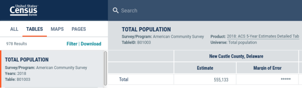
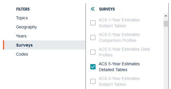
If you’d like to learn more about the census business datasets and understand how to navigate NAICS, check out chapter 8 in my book. I don’t cover the APIs, but I do demonstrate how to use the new data.census.gov and I delve into the concepts behind these datasets in good detail.