distance measures

QGIS Convex Hulls header

Points to Areas with Convex Hulls in GIS

Let’s say you have different sets of points, and each set represents a distinct category of features. Maybe villages where residents speak different languages, or historical events that occurred during different epochs. Beyond plotting and symbolizing the points, perhaps you would like to create areas for each set that represent generalized territory, and you’d like to see how these areas correspond. I’ll demonstrate a few approaches for achieving this, using convex hulls, attribute table calculations, and geoprocessing tools like intersection and union. A convex hull is a minimum bounding polygon, where an area is drawn around all points in a set, where the outermost points serve as vertices for creating boundaries.

I’ll use QGIS for this example, but will mention the corresponding tools in ArcGIS Pro at the end. In QGIS we’ll use the tools that are located within the Processing Toolbox (gear icon on the toolbar). Unlike the shortcut tools under the Vector menu, these tools provide more options and allow us to process multiple files at once.

Steps in QGIS

First, we need either distinct point files for each set of features, or a single file with a categorical variable that distinctly identifies different sets of features. For this example I’ll use three distinct files that I’ve generated using phony sample data. The points are in a projected coordinate system (important!) that’s appropriate for the area I’m mapping.

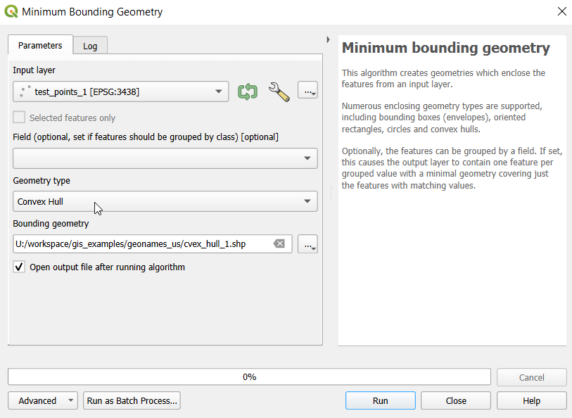
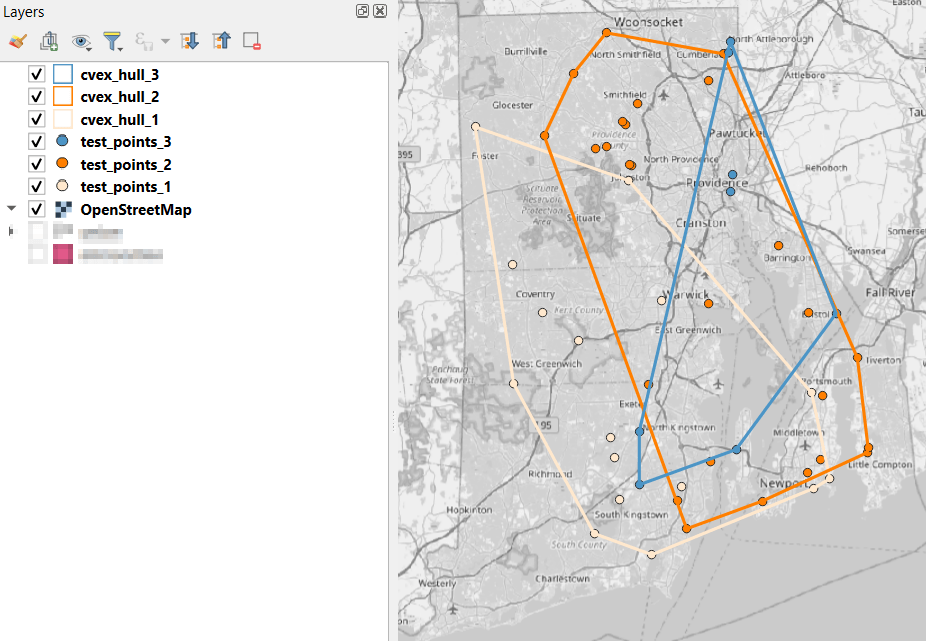
  1. In the QGIS Processing Toolbox, we select the Minimum Bounding Geometry (MBG) tool, and under the Geometry Type specify that we want to create a convex hull. I ran this tool for each file, creating three convex hull files (alternatively, if you had one file with distinct categories, you could use the Field option to generate separate hulls for each category). I’ve symbolized the output below, making the fill hollow and assigning an outline that matches the color of the points. This gives you a good sense for the coverage areas for the points, and how they overlap.
  1. Before running additional tools to explicitly measure overlap, we need to modify the attribute tables of the convex hulls, so we’ll have useful attributes to carry over. The MBG tool creates a new layer with an ID number, area, and perimeter. The ID is set to zero for each hull file, but we should change it to distinctly represent the file / category. With the attribute table open, we can go into an edit mode and type in a new integer value; in this case I’m assigning 1, 2, and 3 to each of the test layers. Alternatively, you could add a new field and assign it a meaningful category value.
  2. The units for area and perimeter match the units used by the map projection of the layer, which is why we want to use a projected coordinate system that uses meters or feet, and not a geographic one (like WGS 84 or NAD 83) that uses degrees. I’m using a state plane system, so the area is in square feet. To convert this to square miles, within the attribute table view I use the Field Calculator to add a new decimal field, and divide the value of the area by 27,878,400 (the number of sq feet in a sq mile; for metric units in meters, we’d divide by 1,000,000 to get sq km). We calculate the area directly from the polygon geometry:
area( @geometry) / 27878400
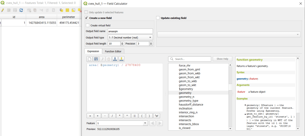
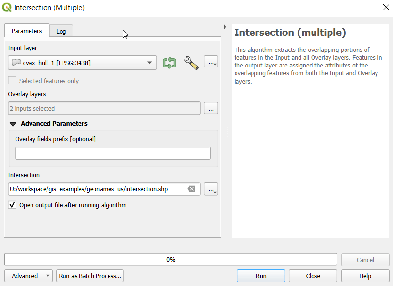
  1. To generate the area of intersection, we go into the Processing tool box and run the Intersection (multiple) tool. The first convex hull is the input layer, while the overlay layers are the other two hull files (in the dialog box, we check the layers we want, and then use the arrow to navigate back to the tool to run it). The output is a new file with polygon(s) that cover the area where all three layers intersect. Its attribute table contains an ID, area, and perimeter field, and we can calculate a new area field in sq miles and see how it compares to the total areas. In my example, the area where all three territories intersect covers about 112 sq miles, while the areas for the individual territories are 512, 563, and 256 sq miles respectively.
  1. To identify distinct areas of overlap between the territories, we return to the Processing toolbox and run the Union (multiple) tool. The dialog is similar to the intersection tool, where the first hull is the union layer and the additional hulls are overlay layers. The output of this tool is a layer with distinct polygons where the hulls coincide. The attribute table for the union layer carries over the attributes from each of the three layers, with columns suffixed with underscores and sequential integers. So if a polygon consists of area covered by hulls 1 and 2, those attributes will be filled in, while the attributes of 3 will be null. As before, we can calculate an area in sq miles for the new polygons. In this case, we’d see that the area covered by hull 1 without any overlapping hulls is 240 sq miles, the largest of all territories.
QGIS Union attribute table
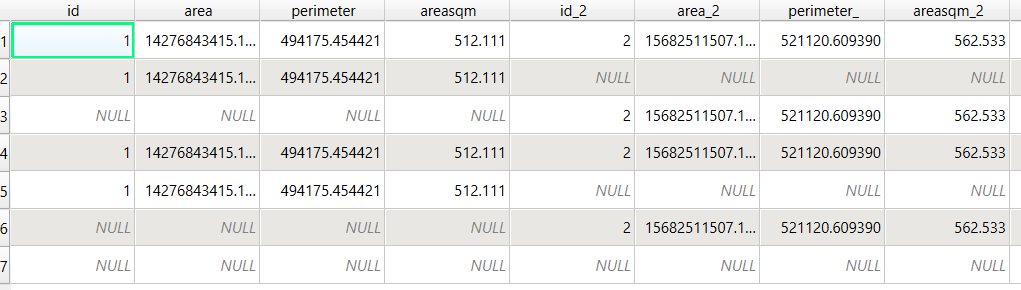
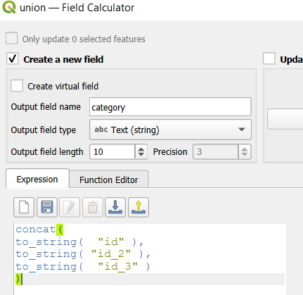
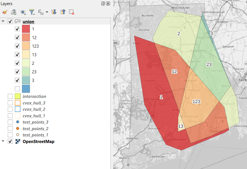
  1. To explicitly categorize these areas, we can add a new field in the attribute table. This will be a text field, where we take the ID numbers, convert them to strings, and concatenate them. In the example above, IDs 1 and 2 would be concatenated to 12, and since the value for 3 is null, no text is appended. (Variation – if you created distinct text-based category fields instead of using the integer IDs, you could concatenate them directly without having to convert them to strings). Using the symbology tool, we can classify the data using these new categories, and can modify the color scheme to something appropriate for displaying the contributions from each area. So a polygon with category 1 includes areas covered by the first convex hull and no others, while category 12 includes areas where hulls 1 and 2 overlapped.
concat(
to_string( "id" ),
to_string( "id_2" ),
to_string( "id_3" )
)

Additional Considerations:

  • With the areas of the individual union pieces, we can compute the percentages of each territory that fall inside and outside various overlapping zones with the field calculator. For example, we can calculate the total area of the union file (which is NOT the sum of each hull, as there’s overlap between them), and then divide each feature by that total to get its percent total. The expression for doing this is below; the numerator has the name of the field that contains the area of each polygon in sq miles, while the denominator includes the calculation for the sum of all parts (alternatively you could use the QGIS Statistics tool to compute this, and hard code the total into the formula):
area_part / (sum(area( geometry(@feature)))/27878400) *100
  • If the idea is to create areas of territory that the points exert influence on, you may want to add a buffer to each hull, to account for the fact that the outer points that form the boundaries will exert influence on both sides of the boundary. Use the Processing – Buffer tool. For the buffer distance, you can use an arbitrary value that makes sense for the circumstances. Or you can generate a relative value that represents a fraction of each convex hull’s area. The output of the buffer tool would then serve as the input to the intersection and union tools.
  • These examples focus on area. If the number of points that falls within the areas is important, you can use the Points in Polygon tool on each of the hulls to count points, and then do the same for the output of the intersection and union tools to get the different points counts for each set of polygons.

ArcGIS Pro Corollaries

Following the same steps above for QGIS, but with ArcGIS Pro:

  1. In the red toolbox, the Minimum Boundary Geometry tool is used to create convex halls. It’s quite similar to the one in QGIS: specify the geometry type, and there is an option to Group (if you have one file with categories). If you leave the Add geometry characteristics box unchecked, it will still compute basic area and perimeter; the checkbox adds a bunch of additional fields.
  2. Unlike QGIS, ArcGIS will not allow you to modify its OBJECTID field. To create a unique value for each hull, you will have to open the attribute table and use the Calculate tool to create a category field (integer or text). To ensure that you can carry it over, in ArcGIS you need to give this column a different name in each hull: cat1, cat2, cat3. Set the value at the bottom in the expression box.
  3. You can use the calculate tool in the attribute table to generate an area column in sqft or sqkm, or use the Calculate Geometry Tool in the toolbox instead. The latter is actually simpler: create a new column, and choose Area and the output units.
  4. The Intersect tool will create the intersection, and functions similarly to QGIS.
  5. The Union tool creates the union, and also functions similarly.
  6. Creating the category field in the union file is a bit more complicated, as ArcGIS assigns values of 0 instead of NULL for non-overlapping polygons. In the Calculate window, with the input file as Union
    and the field as category, change the Expression type to Arcade (ESRI’s scripting language). First, run an expression to concatenate the categories and convert integers to strings (if necessary). Then, replace that expression with a second one that replace the zeros with nothing.
Concatenate(TEXT($feature.cat1)+
TEXT($feature.cat2)+
TEXT($feature.cat3)
)
Replace($feature.category,'0','')
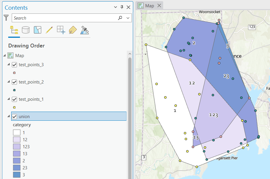
Conclusion

This is a basic approach, appropriate for certain use cases where you want to generate areas from points; particularly when different point sets have a well defined category, so there’s no question of how to group them. Also appropriate where you don’t have – or don’t want – hard boundaries between sets of points and want to see areas of overlap. More sophisticated methods exist for separating points into clusters based on density, distance, and similar attributes, such as K-Means and DB Scan. You can generate non-overlapping territories for individual points using Thiessen / Voronoi polygons, and for points with a sufficiently high density, you can generate rasters with kernel tools.

Route from SciLi to Libraries on OSM

Plotting Routes with OpenRouteService and Python

I made my first foray into network routing recently, and drafted a python script and notebook that plots routes using the OpenRouteService (ORS) API. ORS is based on underlying data from the OpenStreetMap (OSM), and was created by the Heidelberg Institute for Geoinformation Technology, at Heidelberg University in Germany. They publish several routing APIs that include directions, isochrones, distance matricies, geocoding, and route optimization. You can access them via a basic REST API, but they also have a dedicated Python wrapper and an R package which makes things a bit easier. For non-programmers, there is a plugin for QGIS.

Regardless of which tool you use, you need to register for an API key first. The standard plan is free for small projects; for example you can make 2,000 direction requests per day with a limit of 40 per minute. If you’re affiliated with higher ed, government, or a non-profit and are doing non-commercial research, you can upgrade to a collaborative plan that ups the limits. It’s also possible to install OSR locally on your own server for large jobs.

I opted for Python and used the openrouteservice Python module, in conjunction with other geospatial modules including geopandas and shapely. In my script / notebook I read in two CSV files, one with origins and the other with destinations. At minimum both files must contain a header row, and attributes for unique identifier, place label, longitude, and latitude in the WGS 84 spatial reference system. The script plots a route between each origin and every destination, and outputs three shapefiles that include the origin points, destination points, and routes. Each line in the route file includes the ID and names of each origin and destination, as well as distance and travel time. The script and notebook are identical, except that the script plots the end result (points and lines) using geopanda’s plot function, while the Jupyter Notebook plots the results on a Folium map (Folium is a Python implementation of the popular Leaflet JS langauge).

Visit the GitHub repo to access the scripts; a basic explanation with code snippets follows.

After importing the modules, you define several variables that determine the output, including a general label for naming the output file (routename), and several parameters for the API including the mode of travel (driving, walking, cycling, etc), distance units (meters, kilometers, miles), and route preference (fastest or shortest). Next, you provide the positions or “column” locations of attributes in the origin and destination CSV files for the id, name, longitude, and latitude. Lastly, you specify the location of those input files and the file that contains your API key. The location and names of output files are generated automatically based on the input; all will contain today’s date stamp, and the route file name includes route mode and preference. I always use the os module’s path function to ensure the scripts are cross-platform.

import openrouteservice, os, csv, pandas as pd, geopandas as gpd
from shapely.geometry import shape
from openrouteservice.directions import directions
from openrouteservice import convert
from datetime import date
from time import sleep

# VARIABLES
# general description, used in output file
routename='scili_to_libs'
# transit modes: [“driving-car”, “driving-hgv”, “foot-walking”, “foot-hiking”, “cycling-regular”, “cycling-road”,”cycling-mountain”, “cycling-electric”,]
tmode='driving-car'
# distance units: [“m”, “km”, “mi”]
dunits='mi'
# route preference: [“fastest, “shortest”, “recommended”]
rpref='fastest'

# Column positions in csv files that contain: unique ID, name, longitude, latitude
# Origin file
ogn_id=0
ogn_name=1
ogn_long=2
ogn_lat=3
# Destination file
d_id=0
d_name=1
d_long=2
d_lat=3

# INPUTS and OUTPUTS
today=str(date.today()).replace('-','_')

keyfile='ors_key.txt'
origin_file=os.path.join('input','origins.csv') #CSV must have header row
dest_file=os.path.join('input','destinations.csv') #CSV must have header row
route_file=routename+'_'+tmode+'_'+rpref+'_'+today+'.shp'
out_file=os.path.join('output',route_file)
out_origin=os.path.join('output',os.path.basename(origin_file).split('.')[0]+'_'+today+'.shp')
out_dest=os.path.join('output',os.path.basename(dest_file).split('.')[0]+'_'+today+'.shp')

I define some general functions for reading the origin and destination files into nested lists, and for taking those lists and generating shapefiles out of them (by converting them to geopanda’s geodataframes). We read the origin and destination data in, grab the API key, set up a list to hold the routes, and create a header for the eventual output.

# For reading origin and dest files
def file_reader(infile,outlist):
    with open(infile,'r') as f:
        reader = csv.reader(f)    
        for row in reader:
            rec = [i.strip() for i in row]
            outlist.append(rec)
            
# For converting origins and destinations to geodataframes            
def coords_to_gdf(data_list,long,lat,export):
    """Provide: list of places that includes a header row,
    positions in list that have longitude and latitude, and
    path for output file.
    """
    df = pd.DataFrame(data_list[1:], columns=data_list[0])
    longcol=data_list[0][long]
    latcol=data_list[0][lat]
    gdf = gpd.GeoDataFrame(df, geometry=gpd.points_from_xy(df[longcol], df[latcol]), crs='EPSG:4326')
    gdf.to_file(export,index=True)
    print('Wrote shapefile',export,'\n')
    return(gdf)
      
origins=[]
dest=[]
file_reader(origin_file,origins)
file_reader(dest_file,dest)

# Read api key in from file
with open(keyfile) as key:
    api_key=key.read().strip()

route_count=0
route_list=[]
# Column header for route output file:
header=['ogn_id','ogn_name','dest_id','dest_name','distance','travtime','route']

Here are some nested lists from my sample origin and destination CSV files:

[['origin_id', 'name', 'long', 'lat'], ['0', 'SciLi', '-71.4', '41.8269']]
[['dest_id', 'name', 'long', 'lat'],
 ['1', 'Rock', '-71.405089', '41.825725'],
 ['2', 'Hay', '-71.404947', '41.826433'],
 ['3', 'Orwig', '-71.396609', '41.824581'],
 ['4', 'Champlin', '-71.408194', '41.818912']]

Then the API call begins. For every record in the origin list, we iterate through each record in the destination list (in both cases starting at index 1, skipping the header row) and calculate a route. We create a tuple with each pair of origin and destination coordinates (coords), which we supply to the OSR directions API. We pass in the parameters supplied earlier, and specify instructions as False (instructions are the actual turn by turn directions returned as text).

The result is returned as a JSON object, which we can manipulate like a nested Python dictionary. At the first level in the dictionary, we have three keys and values: a bounding box for the route area with a list value, metadata with a dictionary value, and routes with a list value. Dive into route, and the list contains a single dictionary, and inside that dictionary – more dictionaries that contain the values we want!

1st level, dictionary with three keys, the routes key has a single list value
2nd level, the routes list has a single element, another dictionary
3rd level, inside the dictionary in that list element, four keys with route data

The next step is we extract the values that we need from this container by specifying their location. For example, the distance value is inside the first list of routes, inside summary and inside distance. Travel time is in a similar spot, and we take an extra step of dividing by 60 to get minutes instead of seconds. The geometry is trickier as its encoded in some binary line format. We use OSR’s decoding function to turn it into plain text, and shapely to convert it into WKT text; we’ll need WKT in order to get the geometry into a geodataframe, and eventually output as a shapefile. Once we have the bits we need, we string them together as a list for that origin / destination pair, and append this to our route list.

# API CALL
for ogn in origins[1:]:
    for d in dest[1:]:
        try:
            coords=((ogn[ogn_long],ogn[ogn_lat]),(d[d_long],d[d_lat]))
            client = openrouteservice.Client(key=api_key) 
            # Take the returned object, save into nested dicts:
            results = directions(client, coords, 
                                profile=tmode,instructions=False, preference=rpref,units=dunits)
            dist = results['routes'][0]['summary']['distance']
            travtime=results['routes'][0]['summary']['duration']/60 # Get minutes
            encoded_geom = results['routes'][0]['geometry']
            decoded_geom = convert.decode_polyline(encoded_geom) #convert from binary to txt
            wkt_geom=shape(decoded_geom).wkt #convert from json polyline to wkt
            route=[ogn[ogn_id],ogn[ogn_name],d[d_id],d[d_name],dist,travtime,wkt_geom]
            route_list.append(route)
            route_count=route_count+1
            if route_count%40==0: # API limit is 40 requests per minute
                print('Pausing 1 minute, processed',route_count,'records...')
                sleep(60)
        except Exception as e:
            print(str(e))
            
api_key=''
print('Plotted',route_count,'routes...' )

Here is some sample output for the final origin / destination pair, which contains the IDs and labels for the origin and destination, distance in miles, time in minutes, and a string of coordinates that represents the route:

['0', 'SciLi', '4', 'Champlin', 1.229, 3.8699999999999997,
 'LINESTRING (-71.39989 41.82704, -71.39993 41.82724, -71.39959 41.82727, -71.39961 41.82737, -71.39932 41.8274, -71.39926 41.82704, -71.39924000000001 41.82692, -71.39906000000001 41.82564, -71.39901999999999 41.82534, -71.39896 41.82489, -71.39885 41.82403, -71.39870000000001 41.82308, -71.39863 41.82269, -71.39861999999999 41.82265, -71.39858 41.82248, -71.39855 41.82216, -71.39851 41.8218, -71.39843 41.82114, -71.39838 41.82056, -71.39832 41.82, -71.39825999999999 41.8195, -71.39906000000001 41.81945, -71.39941 41.81939, -71.39964999999999 41.81932, -71.39969000000001 41.81931, -71.39978000000001 41.81931, -71.40055 41.81915, -71.40098999999999 41.81903, -71.40115 41.81899, -71.40186 41.81876, -71.40212 41.81866, -71.40243 41.81852, -71.40266 41.81844, -71.40276 41.81838, -71.40452000000001 41.81765, -71.405 41.81749, -71.40551000000001 41.81726, -71.40639 41.81694, -71.40647 41.81688, -71.40664 41.81712, -71.40705 41.81769, -71.40725 41.81796, -71.40748000000001 41.81827, -71.40792 41.81891, -71.40794 41.81895)']

Finally, we can write the output. We convert the nested route list to a pandas dataframe and use the header row for column names, and convert that dataframe to a geodataframe, building the geometry from the WKT string, and write that out. In contrast, the origins and destinations have simple coordinates (not in WKT), and we create XY geometry from those coordinates. Writing the geodataframe out to a shapefile is straightforward, but for debugging purposes it’s helpful to see the result without having to launch GIS. We can use geopandas’s plot function to draw the resulting geometry. I’m using the Spyder IDE, which displays plots in a dedicated window (in my example the coordinate labels for the X axis look strange, as the distances I’m plotting are small).

# Create shapefiles for routes
df = pd.DataFrame(route_list, columns=header)
gdf = gpd.GeoDataFrame(df, geometry=gpd.GeoSeries.from_wkt(df["route"]),crs = 'EPSG:4326')
gdf.drop(['route'],axis=1,inplace=True) # drop the wkt text
gdf.to_file(out_file,index=True)
print('Wrote route shapefile to:',out_file,'\n')

# Create shapefiles for origins and destinations
ogdf=coords_to_gdf(origins,ogn_long,ogn_lat,out_origin)
dgdf=coords_to_gdf(dest,d_long,d_lat,out_dest)

# Plot
base=gdf.plot(column="dest_id", kind='geo',cmap="Set1")
ogdf.plot(ax=base, marker='o',color='black')
dgdf.plot(ax=base, marker='x', color='red');

In a notebook environment we can employ something like Folium more readily, which gives us a basemap and some basic interactivity for zooming around and clicking on features to see attributes. Implementing this was a more complex than I thought it would be, and took me longer to figure out compared to the routing process. I’ll return to those details in a subsequent post…

In my sample data (output rendered below in QGIS) I was plotting fastest driving distance from the Brown University Sciences Library to the other libraries in our system. Compared to Google or Apple Maps the result made sense, although the origin coordinates I used for the SciLi had an impact on the outcome (assumed you left from the loading dock behind the building as opposed to the front door as Google did, which produces different routes in this area of one-way streets). My real application was plotting distances of hundreds of miles across South America, which went well and was useful for generating different outcomes using fastest or shortest route.

Take a look at the full script in GitHub, or if programming is not your thing check out the QGIS plugin instead (activate in the Plugins menu, search for OSR). Remember to get your API key first.

Least Cost Paths in QGIS and GRASS

Cost Surfaces and Least Cost Paths in QGIS and GRASS

In this post I’ll demonstrate how to create least cost paths using QGIS and GRASS GIS, and in doing so will describe how a cost surface is constructed. In a surface analysis, you model movement across a grid whose values represent friction encountered in moving across it. In computing a least cost path, you’re seeking an optimal route from an origin to the closest destination, where ‘close’ incorporates distance and ease of movement across that surface. These kinds of analyses are often conducted in the environmental sciences, in modeling the movement of water across terrain, and in zoology in predicting migration paths for land-based animals.

In this example the idea was to chart the origin of settlements and possible trade routes in ancient history. In applications where we’re studying human activity, network analysis is typically used instead. Networks use geometry, where a node is a place or person, and connections between nodes are indicated with lines. Lines typically have a value associated with them that identify either the strength of a connection, or conversely friction associated with moving between nodes. The idea for this project was to identify how networks formed, so the surface analysis served as a proto-network analysis. While there were roads and maritime routes in pre-modern times, these networks were weaker and less dense. Charting movement over a surface representing terrain could provide a decent approximation of routes (but if you’re interested in ancient Roman network routing, check out the ORBIS project at Stanford).

This example stems from a project I was helping a PhD student with; I don’t want to replicate his specific study, so I’ve modified the data sources and area of focus to model movement between large settlements and stone quarries in the ancient Roman world. My goal is to demonstrate the methods with a plausible example; if we were doing this as part of an actual study, we would need to be more discriminating in selecting and processing our data.

Preliminary Work

The Pleiades project will serve as our source for destinations; it’s an academic gazetteer that includes locations and place names for the ancient and early medieval world, stretching from Europe and North Africa through the Middle East to India. It’s published in many forms, and I’ve downloaded the Pleiades Data for GIS in a CSV format. Using QGIS, I used the Add Delimited Text tool to plot the places.csv to get all of the locations, and joined that file to the places_place_type.csv file which contains different categories of places. I used Select by Attributes to get locations classified as quarries, and exported the selection out to a geopackage.

The Pleiades data includes a category for settlements, but there are about ten thousand of these and there isn’t an easy way to create a subset of the largest places. So I opted to use Hanson’s dataset of the largest settlements in the ancient Roman world to serve as our source for origins (about 1,400 places). This data was packaged in an Excel file; I plotted the coordinates using the Create Points Layer from Table tool in QGIS and converted the result to a geopackage. For testing purposes, I selected a subset of ten major cities and saved them in a separate layer: Athenae, Alexandria (Aegyptus), Antiochia (Syria), Byzantium, Carthago, Ephesus, Lugdunum, Ostia, Pergamum, Roma.

For the friction grid, I downloaded a geoTIFF of the Human Mobility Index by Ozak. The description from the project:

“The Human Mobility Index (HMI) estimates the potential minimum travel time across the globe (measured in hours) accounting for human biological constraints, as well as geographical and technological factors that determined travel time before the widespread use of steam power.”

There are three separate grids that vary in extent based on the availability of seafaring technology. I chose the grid that incorporates seafaring prior to the advent of ocean-going ships, which is appropriate for the Mediterranean world during the classical era. The HMI is a global grid at 925 meter resolution. To minimize processing time, I clipped it to a bounding box that encompasses the area of study. The grid is in the World Cylindrical Equal Area system; I reprojected it to WGS 84 to match the rest of the layers. As long as we’re not measuring actual distances, we don’t need to worry about the system we’re using (but if we were, we’d use an equidistant system). Since the range of values is small and it’s hard to see differences in cell values, I symbolized the grid as single-band psuedo color and used a quantiles classification scheme with 12 categories.

Lastly, I grabbed some modern country boundaries from Natural Earth to serve as a general frame of reference. A screenshot of the workspace is below:

Least Cost Path in QGIS

QGIS has a third-party plug-in for doing a least cost path analysis, which works fine as long as you don’t have too many origin points. Go to Plugins > Manage and Install Plugins > Least Cost Path to turn it on. Then open the Processing toolbox and it will be listed at the bottom. See the screenshot below for the tool’s menu. The Cost raster layer is the friction surface, so the human mobility index in this example. The start points are the ten major cities and the end points are the quarries. The start-point layer dialog only accepts a single point; if you have multiple points, hit the green circular arrow button to iterate across all of them. There’s a checkbox for connecting the start point to just the nearest end point (as opposed to all of them). Save the output to a geopackage.

It took about five minutes to run the analysis and iterate across all ten points. Each path is saved in a separate file, but since they have an identical structure I subsequently used Vector > Data Management Tools > Merge Vector Layers to combine them into one file. The attribute table records the end point ID (for the quarry) and the accumulated cost, but does not include the origin ID; this ID is the number 1 repeated each time, as the tool was iterating over the origin points. We can see the result below; for Athens and Ephesus in the south, land routes were shortest, whereas for Pergamum and Byzantium in the north it was easier (distance and friction-wise) to move across the sea.

While this worked fine for ten cities, it would take a considerable amount of time to compute paths for all 1,400. The problem here is that the plugin was designed for one point at a time. Let’s outline the process so we can understand how alternatives would work.

Cost Surface Analysis

To calculate a least cost path, the first step is to create a cost surface, where we take our friction grid and the destinations and calculate the total cost of movement across all cells to the nearest destination. First, the destinations are placed on the grid, and they become the grid sources. Then, the accumulated cost of moving from each source to its adjacent cells is calculated. For horizontal and vertical movement, it’s the sum of the friction values divided by two, and for diagonal movement it’s the sum of the friction values divided by two then multiplied by 1.4142. Once those calculations are performed, those adjacent cells are assigned to each source. Next, the lowest accumulated cost cell in the grid is identified, the cost for moving to its unassigned neighbors is calculated, and these cells are assigned to the same source. This process is repeated by cycling through the lowest accumulated value until all calculations for the grid are finished. Illustrated in the example below, which I derived from Lloyd’s Spatial Data Analysis (2010) pp. 165-168.

For each cell, three items are recorded, and are saved either as separate bands in one raster, or in three separate raster files:

  1. Accumulated cost of moving to that cell from the nearest source
  2. Assignment or allocation of the cell to its source (the nearest one to which it “belongs”)
  3. A vector that indicates direction from that source

With these cost surfaces, we can take the second step of calculating the least cost path. We place a number of starting points onto this surface, and each point is assigned to the closest destination based on where its grid cell was allocated. The direction to that destination is traced backward using the direction grid, and the total cost of movement is taken from the accumulated cost surface.

Knowing how this process works, there are two practical conclusions we can draw. First, when computing the cost surface, you use your destinations (not the origins) as the source for the cost surface. You use the origins as the start points for the least cost path. Second, there’s no need to recalculate the cost surface for every origin point; you only need to do this once. That’s why the QGIS plugin took so long; it was recomputing the cost surface each time. Knowing this, we can use GRASS GIS to compute the paths, as it’s designed to compute the surface just once (and it’s data structure will also boost performance a bit).

Cost Surface Analysis in GRASS

GRASS GIS comes bundled with QGIS. While it’s possible to run a number of GRASS tools directly within QGIS, it’s a bit undesirable as you’re not able to access the full range of parameters or options for each GRASS command. I opted to create the GRASS environment in QGIS, and loaded all the necessary data into the GRASS format. Then, I flipped over to the GRASS GUI to do the analysis.

GRASS uses a distinct database structure and file format, and we need to create a GRASS workspace and load our data into that database in order to use the cost surface tools. I followed the steps in the QGIS manual for creating a GRASS environment and loading data into a GRASS database. Once you create the database and mapset, you use the QGIS Browser to browse to the grassdata folder and designate your new mapset as your working mapset (mapsets have the little green grass icon beside them). With the GRASS tools open, I used v.in.ogr.qgis to load my my cities and quarries layers into this mapset, and r.in.gdal.qgis to load the mobility index (if these layers weren’t already in your QGIS project, you’d use the tools that don’t have the qgis suffix, i.e. v.in.ogr).

After exiting QGIS and launching GRASS, you select the mapset under the grassdata database at the top, right click and choose Switch mapset, and choose the mapset you want to work with (if you don’t see it, hit the database icon to browse and connect to the grassdata folder). You can display the layers in the GRASS window to visualize them, but it’s not necessary for running the tools. In the tool menu on the right, search for the Cost surface tool, r.cost, and choose the following options:

  • Required: input raster map with grid cell cost is the human mobility index, and output raster is cost_surface
  • Optional outputs: output raster with nearest start point as allocation_surface, output raster with movement as direction_surface
  • Start: vector starting points for the cost surface are the destinations, the quarries
  • Optional: check verbose output (to get more details on errors)
GRASS GIS GUI and r.cost

Running this operation on all 1,400 cities took a matter of seconds, and all three rasters described in the previous section were generated: cost, allocation, direction (shown below).

Using these outputs, we can run the Least cost route or flow tool, which is called r.drain (as it’s often used in earth sciences to chart the path that water will drain based on elevation).

  • Required: Name of input elevation or cost surface raster is cost_surface, Name of output raster path: is path_raster
  • Cost surface: check the Input raster map is a cost surface box, Name of input movement direction raster is direction_surface
  • Start: Name of starting points vector map: are the origins (cities)
  • Path settings: choose ONE option that you’d like to record (or none)
  • Optional: check Verbose mode, Name for output drain vector is path_vector

This also took mere seconds to complete (!) and generated the paths from each origin (city) to the closet destination (quarry) over the surface as both raster cells and vector lines. The output in GRASS is shown below.

Least cost path output in GRASS GIS

At this stage, we can hop back into QGIS, and load these output paths into our original project to symbolize and study what’s going on. Notice the settlements in northeastern Italy and along the Dalmatian coast; for many of them the least cost path is to a quarry across the sea rather than through rugged mountainous terrain. Even though some quarries in the mountains may be closer in actual distance, it’s a tougher path to travel.

Conclusion

The benefit of using GRASS is that we can run these processes fairly quickly for large datasets. The GRASS commands can also be compiled into a batch script, so you can create a documented and automated process instead of having to drill through multiple menus.

A big downside of the GRASS tools for this analysis is that the resulting vector paths contain no information about the origin or destination points, and only the raster path output carries along values. You might be able to generate this information through some extra steps; using the QGIS field calculator, you can get the coordinates for the start point and end point of each path and add them explicitly to the attribute table. Then take those coordinates, and for the start point of the line select the closest city and get its attributes, and for the end point select the closet quarry and get its attributes. I say “closest” because the vector paths don’t snap perfectly to the start and end points. Modifying the resolution of the human mobility index to make it coarser (fewer cells) might help to resolve this, or converting the origin and destination points to a raster of the same resolution as the index. Alternatively, if you incorporate the GRASS commands into a Python script, you could iterate over the origins in the least cost path analysis and record the origin IDs as you step through.

I haven’t worked all the pieces, but hopefully this will be useful for those of you who are interested in conducting a basic cost surface analysis in open source. The student I was helping was interested in measuring the density of the paths across a grid, so this process worked for him as he didn’t need to associate the paths with origins and destinations. Beyond FOSS GIS, ArcGIS Pro has a full suite of tools for cost surface analysis, and the underlying methods and logic are the same.

Average Distance to Public Libraries in the US

A few months ago I had a new article published in LISR, but given the absurd restrictions of academic journal publishing I’m not allowed to publicly post the article, and have to wait 12 months before sharing my post-print copy. It is available via your local library if they have a subscription to the Science Direct database (you can also email me to request a copy). .

Citation and Abstract

Regional variations in average distance to public libraries in the United States
F. Donnelly
Library & Information Science Research
Volume 37, Issue 4, October 2015, Pages 280–289
http://dx.doi.org/10.1016/j.lisr.2015.11.008

Abstract

“There are substantive regional variations in public library accessibility in the United States, which is a concern considering the civic and educational roles that libraries play in communities. Average population-weighted distances and the total population living within one mile segments of the nearest public library were calculated at a regional level for metropolitan and non-metropolitan areas, and at a state level. The findings demonstrate significant regional variations in accessibility that have been persistent over time and cannot be explained by simple population distribution measures alone. Distances to the nearest public library are higher in the South compared to other regions, with statistically significant clusters of states with lower accessibility than average. The national average population-weighted distance to the nearest public library is 2.1 miles. While this supports the use of a two-mile buffer employed in many LIS studies to measure library service areas, the degree of variation that exists between regions and states suggests that local measures should be applied to local areas.”

Purpose

I’m not going to repeat all the findings, but will provide some context.

As a follow-up to my earlier work, I was interested in trying an alternate approach for measuring public library spatial equity. I previously used the standard container approach – draw a buffer at some fixed distance around a library and count whether people are in or out, and as an approximation for individuals I used population centroids for census tracts. In my second approach, I used straight-line distance measurements from census block groups (smaller than tracts) to the nearest public library so I could compare average distances for regions and states; I also summed populations for these areas by calculating the percentage of people that lived within one-mile rings of the nearest library. I weighted the distances by population, to account for the fact that census areas vary in population size (tracts and block groups are designed to fall within an ideal population range – for block groups it’s between 600 and 3000 people).

Despite the difference in approach, the outcome was similar. Using the earlier approach (census tract centroids that fell within a library buffer that varied from 1 to 3 miles based on urban or rural setting), two-thirds of Americans fell within a “library service area”, which means that they lived within a reasonable distance to a library based on standard practices in LIS research. Using the latest approach (using block group centroids and measuring the distance to the nearest library) two-thirds of Americans lived within two miles of a public library – the average population weighted distance was 2.1 miles. Both studies illustrate that there is a great deal of variation by geographic region – people in the South consistently lived further away from public libraries compared to the national average, while people in the Northeast lived closer. Spatial Autocorrelation (LISA) revealed a cluster of states in the South with high distances and a cluster in the Northeast with low distances.

The idea in doing this research was not to model actual travel behavior to measure accessibility. People in rural areas may be accustomed to traveling greater distances, public transportation can be a factor, people may not visit the library that’s close to their home for several reasons, measuring distance along a network is more precise than Euclidean distance, etc. The point is that libraries are a public good that provide tangible benefits to communities. People that live in close proximity to a public library are more likely to reap the benefits that it provides relative to those living further away. Communities that have libraries will benefit more than communities that don’t. The distance measurements serve as a basic metric for evaluating spatial equity. So, if someone lives more than six miles away from a library that does not mean that they don’t have access; it does means they are less likely to utilize it or realize it’s benefits compared to someone who lives a mile or two away.

Data

I used the 2010 Census at the block group level, and obtained the location of public libraries from the 2010 IMLS. I improved the latter by geocoding libraries that did not have address-level coordinates, so that I had street matches for 95% of the 16,720 libraries in the dataset. The tables that I’m providing here were not published in the original article, but were tacked on as supplementary material in appendices. I wanted to share them so others could incorporate them into local studies. In most LIS research the prevailing approach for measuring library service areas is to use a buffer of 1 to 2 miles for all locations. Given the variation between states, if you wanted to use the state-average for library planning in your own state you can consider using these figures.

To provide some context, the image below shows public libraries (red stars) in relation to census block group centroids (white circles) for northern Delaware (primarily suburban) and surrounding areas (mix of suburban and rural). The line drawn between the Swedesboro and Woodstown libraries in New Jersey is 5-miles in length. I used QGIS and Spatialite for most of the work, along with Python for processing the data and Geoda for the spatial autocorrelation.

Map Example - Northern Delaware

The three tables I’m posting here are for states: one counts the 2010 Census population within one to six mile rings of the nearest public library, the second is the percentage of the total state population that falls within that ring, and the third is a summary table that calculates the mean and population-weighted distance to the nearest library by state. One set of tables is formatted text (for printing or just looking up numbers) while the other set are CSV files that you can use in a spreadsheet. I’ve included a metadata record with some methodological info, but you can read the full details in the article.

In the article itself I tabulated and examined data at a broader, regional level (Northeast, Midwest, South, and West), and also broke it down into metropolitan and non-metropolitan areas for the regions. Naturally people that live in non-metropolitan areas lived further away, but the same regional patterns existed: more people in the South in both metro and non-metro areas lived further away compared to their counterparts in other parts of the country. This weekend I stumbled across this article in the Washington Post about troubles in the Deep South, and was struck by how these maps mirrored the low library accessibility maps in my past two articles.