NOTE – in mid-2021 the GeoBlacklight metadata standard was refined and renamed as the OpenGeoMetadata Aardvark Metadata Schema. The documentation for the standard was moved from the GB to the OGM GitHub repo.
During the COVID-19 lock down this past spring, I took the opportunity to tackle a project that was simmering on my back burner for quite a while: creating a coherent metadata standard for describing all of the GIS data we create in the lab. For a number of years we had been creating ISO 19115 / 19139 metadata records in XML, which is the official standard. But the process for creating them was cumbersome and I felt it provided little benefit. We don’t have a sophisticated repository where the records are part of a search and retrieval system, and that format wasn’t great for descriptive documentation either, i.e. people weren’t reading or referring to the metadata to learn about the datasets.
We were already creating basic Dublin Core (DC) records for our spatial databases and non-spatial data layers, so I decided to create some in-house guidelines and build processes and scripts for creating all of our metadata in DC, while adhering to guidelines and best practices established by the GeoBlacklight community. I’ll describe my process in this post, and hopefully it should be useful for others who are looking to do similar work. I’ll mention some resources for learning more about geospatial metadata in the conclusion.
All of the metadata documentation and scripts I’ve created are available on GitHub. I’ll add a few snippets of code here and there to illustrate,
Out With the Old
FGDC and ISO 19115 / 19139 have long been the standards for creating geospatial metadata and expressing it in XML. The ISO standard has eclipsed the FGDC standard, but some institutions continue to use FGDC for legacy reasons. Since ISO was the standard, I decided that we should use it for all the layers we create in the lab. So why am I abandoning it?
The ISO standard is enormous and complex. Even though we were using just the required elements in the North American Profile, there were still over 100 fields that we had to enter. Many of them seemed silly, like having to input a name and mailing address for our organization for every instance where we were a publisher, distributor, creator, etc. We were creating the records in the ArcCatalog, which only permits you to create and edit records using the ArcGIS metadata standard. You have to export the results out to ISO, but if you have changes to make you need to edit the original ArcGIS metadata, which forces you to keep two copies of every record. The metadata can be easily viewed in ArcCatalog, but not in other software. Creating your own stylesheet for displaying ISO records is a real pain, because there are dozens of namespaces and lots of nesting in the XML. So we ended up printing the styled records from ArcCatalog as PDFs (ugh), to include alongside the XML. Processing and validating the records to our own standards was equally painful.
In short, metadata creation became a real bottleneck in our data creation process, and the records didn’t serve a useful purpose for either search or description. Each record was about six pages long, and at least two-thirds of the information wasn’t relevant for people who were trying to understand our data.
In with the New
Dublin Core (DC) is a basic, open-ended metadata standard that was created in the mid 1990s, and has been adopted by numerous libraries and archives for documenting collections. There is a set of core elements and an additional set of terms that refine these elements. For example, there is a core Coverage element intended for describing time and place, but then there are more specific DC terms for Temporal and Spatial description. DC hasn’t been widely used for geospatial metadata because it’s not able to express all of the details that are important to those datasets, such as coordinate reference systems, resolution, and scale.
At least that’s what I thought. GeoBlacklight is an open source search and discovery platform for GIS data which relies on metadata records to power the platform. It was developed at Stanford and is used by several universities such as NYU and Cornell. A working group behind the project created and adopted a GeoBlacklight Metadata Schema (GB) which uses a mix of DC elements and GB-specific elements that are necessary for that platform. GB metadata is stored in a JSON format.
The primary aim of the standard is to provide records that aid searching, and there is less of an emphasis on fully describing the datasets for the purpose of providing documentation. But for my purposes, it was fine. I could adopt a subset of the DC elements and terms that I felt were necessary for describing our resources, while keeping an eye on the GB standard and following it wherever I could. If there was a conflict between what we wanted to do and the GB standard, I made sure that I could crosswalk one to the other. I would express our records in XML, and would write a script to transform them to the GB standard in a JSON format. That way, I can share our data and metadata with NYU, which has a GB-backed spatial data repository and re-hosts several of our datasets.
Data Application Profile
The first step was to establish our in-house guidelines. I created a data application profile to specify the DC elements we would use, which are required versus optional, and whether they can repeat or not. For example, we require a Title and Creator element, where there can be only one title but multiple creators (as more than one person may have created the resource). We also use the Contributor element to reference people who had some role in creating the dataset, but not as significant as the creator. This element is optional, as there might not be a contributor.
For some of the elements we require specific formatting, while for others we specify a set of controlled terms that must be used. For the Title, we follow Open Geoportal best practices where the title is written as: Layer Name, Place, Date (OGP is a separate but related geospatial data discovery platform and community). Publication dates are written as YYYY-MM. For the Subject element, we use the ISO 19115 categories that are commonly used for describing geospatial data. These are useful for filtering records by topic, and are much easier to consistently implement than Library of Congress Subject Headings. In some cases I adopted elements and vocabulary that were required by GB, such as the Provenance field which is used by GB to record the name of the institution that holds the dataset.
Snippet of an XML metadata record:
<title>Real Estate Sales, New York NY, 2019</title>
<creator>Frank Donnelly</creator>
<creator>Anastasia Clark</creator>
<subject>economy</subject>
<subject>planningCadastre</subject>
<subject>society</subject>
<subject>structure</subject>
In other cases I went contrary to the GB standard, but kept an eye on how to satisfy it so when records are crosswalked from our DC standard in XML to the GB standard in JSON, the GB records will contain all the required information. I used the DC Medium element to specify how the GIS data was represented (point, line, polygon, raster, etc), which is required as a non-DC element in GB records. I used the Source element to express the original data sources we used for creating our data, which is something that’s important to us. GB doesn’t use the Source element in this way – so when our records are crosswalked this information will be dropped. I used Coverage for expressing place names from Geonames, and Spatial to record the bounding box for the features using the DC Box format. I also used The Spatial field as a way of expressing the coordinate reference system for the layer: the coordinates and system name published in the record are for the system the layer uses. When this information gets crosswalked to a GB record, the data in Coverage will be transferred to Spatial (as GB uses this DC field for designating place names), and the Spatial bounding box data gets migrated and transformed to a GB-specific envelope element (in GB, the bounding box is used for spatial searching and is expressed in WGS 84).
Creating Records and Expressing them in XML
I created a blank XML template that contains all our required and optional elements, with some sample values to indicate how the elements should be populated. If we are creating new records from scratch, we can copy the template and fill it in using a plain text editor. Alternatively we can also use the Dublin Core Metadata Generator, but in using that we’d have to be careful to follow our DAP, selecting just our required elements and omitting ones that we don’t use. All of our elements are expressed under a single root element called “metadata”. While it is common to prefix DC elements with a namespace, we do NOT include these namespaces because it makes validating the records a pain… more about that in the next section.
In most cases, we won’t be creating records from scratch but will be modifying existing ones, and only a handful of the elements would need to be updated in any given year. To this end, I wrote two scripts that make copies of specific records, one for each year or time period (for one feature that repeats over many years – one file to many), and one for each file name (for a series of different layers produced for one time period – one file to one file). That way, we can edit the copies and change just the fields that need updating.
The process of updating the records is going to vary with each series and with each particular iteration. I wrote some Python functions that can be used repeatedly, and import these into scripts that are custom designed for each dataset. I use the ElementTree module to parse the XML and update specific fields. For elements that require updated values, I either hard code them into the script or read them from a JSON file that I construct. For example, to update our real estate sales layers I took the file for the most recent year and made copies of it, named for each year in the past. Then I created a JSON file that’s read into a Python dictionary, and using the year in the file name as the key, elements for: year issued, year published, creator, and contributor in the XML are modified using the dictionary values. In some cases the substring of an element must be changed, such as the year that appears at the end of the Title field. In other cases an entire value can simply be swapped out.
A portion of a json file is below, where year is the key and value is a dictionary that contains element name as key, and value is element text / value to be updated:
{
"2018":{"issued":"2019-05","creator":["Anastasia Clark","Frank Donnelly"],"contributor":["Chris Kim"]},
"2017":{"issued":"2018-10","creator":["Anastasia Clark","Frank Donnelly"],"contributor":["Abigail Andrews"]},
"2016":{"issued":"2017-05","creator":["Anastasia Clark"],"contributor":["Frank Donnelly","Janine Billadello"]},
}
Several files called “real_property_sales_nyc_YEAR.xml” are read in. These files are all copies of data for the most recent year (2019), but YEAR in the file name is substituted with each year of data that we have (2018, 2017, etc). The script reads in the year from the file name, and updates the appropriate elements using that year as the key (in the actual code the functions are imported from a separate file so they can be used in multiple scripts). With ElementTree: parse the xml file to save it as a tree object, then getroot to get the root element of the tree, which allows you to find specific elements (like the title element) and get the text value of that element (the actual title), so you can modify the value:
import xml.etree.ElementTree as ET
def esimple(root,elem,value):
"""Replace the value of an element"""
e=root.find(elem)
e.text=value
def esubstring(root,elem,oldstring,newstring):
"""Replace a portion (substring) of the value of an element"""
e=root.find(elem)
e.text=e.text.replace(oldstring,newstring)
with open(json_update_file) as jfile:
updates = json.load(jfile)
for file in os.listdir(infolder):
if file[-4:]=='.xml':
xfilein=os.path.join(infolder,file)
year=file[-8:-4] #assumes year is at end of file name
tree = ET.parse(xfilein)
root = tree.getroot()
esimple(root,'temporal',year)
esimple(root,'issued',updates[year]['issued'])
esubstring(root,'title','2019',year)
...
Validating Records
Since I’m already operating within Python, I decided to use a 3rd party Python module called xmlschema to validate our records. It’s simple and works quite nicely, but first we need to have a schema. An XML schema or XSD file is an XML file that contains instructions on how our XML metadata should be structured: all the elements we use, whether they are required or not, whether they can repeat or not, the order in which they must appear, and whether there are controlled vocabularies. I hard-coded shorter vocabs like the ISO categories and many of the GB requirements into the schema, but I didn’t include absolutely everything. Since we’re a small shop that makes a limited amount of metadata, we’ll still be checking the records manually.
The Python validator script checks for well formed-ness first (i.e. every open tag has a closing tag), and then proceeds to check the record against the schema file. If it hits something that’s invalid, it stops. I wrote the script as a batch process, so if one file fails it moves on to the next one. It produces an error report, and we make the corrections and go back and try validating again until everything passes.
In the snippet below, we read in the schema file and a folder of records to be validated. myschema.is_valid(file) tests whether the schema is valid or not. If it’s valid (True) I perform some other check (not shown), and if that turns out OK then we have no problems. Otherwise if my check fails, or the schema returns as not valid (False), record the problem and move on to the next file. Problems are printed to screen, and other status messages are output (not shown):
import xmlschema as xmls
import os
schemafile=os.path.join('bcgis_dc_schema.xsd')
xmlfolder=os.path.join('projects','nyc_real_estate','newfiles')
problems={}
noproblems=[]
my_schema = xmls.XMLSchema(schemafile)
for file in os.listdir(xmlfolder):
if file[-4:]=='.xml':
filepath=os.path.join(xmlfolder,file)
my_xml = xmls.XMLResource(filepath)
test=my_schema.is_valid(my_xml)
if test==True:
msg=spatial_check(my_xml)
if msg==None:
noproblems.append(file)
else:
problems[file]=msg
else:
try:
my_schema.validate(my_xml)
except xmls.XMLSchemaException as e:
problems[file]=e
continue
if len(problems)&amp;gt;0:
print('***VALIDATION ERRORS***\n')
for k, v in problems.items():
print(k,v)
else:
pass
Creating the schema was an area where I ran into trouble, because I initially tried to refer to the DC namespaces in my records and kept all of the namespace prefixes with the elements, i.e. dc:title instead of title. This seemed like the “right” thing to do. It turns out that schema creation and validation for XML records with multiple namespaces is a royal pain; you have to create multiple schemas for each namespace, which in this case would mean three: DC elements, DC terms, and my own root metadata element. Then I’d have to write all kinds of stuff to over-ride the default DC schema files, because they were designed to be flexible: the only requirement is that just the listed DC elements and terms can appear. My requirements are much more stringent, as I wanted to use a subset of the DC elements and impose restrictions to insure consistency. I watched countless YouTube videos on XML schemas and read several tutorials that didn’t address this complexity, and what I did find suggested that it was going to be arduous.
Ultimately I decided – why bother? I jettisoned the namespaces from our records, and have yet another script for stripping them out of records (for older records where we had included namespaces). As long as I have a solid DAP, am following best practices consistently, am using vocabularies that others are using, and we validate and check our records, others should be able to interpret them and either ingest or transform them if they need to.
Styling the Records
While XML is fine for search and data exchange, it’s not friendly for humans to read, so it’s a good idea to apply a stylesheet to render the XML in a readable form in a web browser. XLST stylesheets give you lots of control, as you can actually process and transform the underlying XML to display what you want. But to my dismay, this was also needlessly complicated. Searching around, I discovered that many web browsers had deprecated the display of XML via XLST stylesheets stored locally for security reasons, which makes development cumbersome. I also got the sense that this is an atrophying technology; most of the references I found to XSLT were 10 to 20 years old.
So, I took a simpler route and created a CSS stylesheet, which can style XML essentially the same way that it styles HTML. You must display all of the underlying data in the XML file and your control is limited, but there are enough tweaks where you can insert labels, and vary the display for single items versus lists of items. I keep the stylesheet stored on our website, and as part of the metadata creation process a link to it is embedded in each of our records. So when you open the XML file in a browser, it looks to the online CSS file and renders it. The XML snippet at the beginning of this post looks like the image below, when a user clicks on the file to view it:
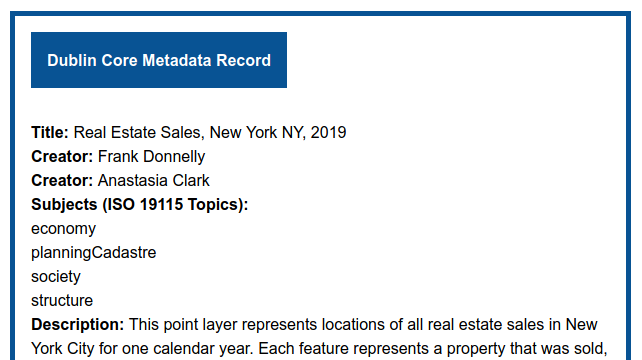
You can access this actual metadata record on our webserver via the Baruch Geoportal.
Crosswalk DC XML TO GB JSON
Migrating the DC XML records to GB JSON was actually straightforward, using Python and a combination of the ElementTree and JSON modules. I walked each of our elements over to its corresponding GB element, and made modifications when needed using the ElementTree functions and methods mentioned previously; I find each element in our XML and save its value in a dictionary using the GB element name as the key, and at the end I write the items out to JSON. In some cases elements from our records are dropped if there isn’t a suitable counterpart. The bounding box element was trickiest, as I had to convert the northing and easting coordinate format used by DC box into a standard OGC Envelope structure, and transform the CRS from whatever the layer uses to WGS 84. I used the pyproj module to do both. Some of the elements are left blank, because I’d have to coordinate with my colleagues at NYU for filling those values, like the unique id or “slug” that’s native to their repository.
Conclusion
You should always create metadata and rely on existing standards and vocabulary to the extent possible, but create something that works for you given your circumstances. Figure out whether your metadata serves a discovery function or a documentation function, or some combination of both. Create a clear set of rules that you can implement that will provide useful information to your data users, without becoming a serious impediment to your data creation process. Creating metadata does take time and you need to budget for it accordingly, but don’t waste time (like I was) dealing with clunky metadata creation software and lots of information that will largely go unused, simply because it’s “the right thing to do”. Ideally, whatever you create should be consistent and flexible enough that you can write some code to transfer it to a different standard or format if need be.
For more information about GeoBlacklight metadata, take a look at this Code4Lib article about the GB metadata schema written by the developers a few years back, but consult the current standard (which has changed a bit since the article was written). Another Code4Lib article reviews tools for working with geospatial metadata that include GUI-solutions, XSLT, and Python with ElementTree. My colleague Andrew Battista at NYU has written a post about authoring GB metadata; they use Omeka as a user-friendly front end for creating their records.


You must be logged in to post a comment.