In an earlier post, I described how to summarize and extract raster temperature data using GIS. In this post I’ll demonstrate some alternate methods using spatial Python. I’ll describe some scripts I wrote for batch clipping rasters, overlaying them with point locations, and extracting raster values (mean temperature) at those locations based on attributes of the points (a matching date). I used a number of third party modules, including geopandas (storing vector data in a tabular form), rasterio (working with raster grids), shapely (building vector geometry), matplotlib (plotting), and datetime (working with date data types). Using Anaconda Python, I searched for and added each of these modules via its package handler. I opted for this modular approach instead of using something like ArcPy, because I don’t want the scripts to be wedded to a specific software package. My scripts and sample data are available in GitHub; I’ll add snippets of code to this post for illustration purposes. The repo includes the full batch scripts that I’ll describe here, plus some earlier, shorter, sample scripts that are not batch-based and are useful for basic experimentation.
Overview
I was working with a medical professor who had point observations of where patients lived, which included a date attribute of when they had visited a clinic to receive certain treatment. For the study we needed to know what the mean temperature was on that day, as well as the temperature of each day of the preceding week. We opted to use daily temperature data from the PRISM Climate Group at Oregon State, where you can download a raster of the continental US for a given day that has the mean temperature (degrees Celsius) in one band, at 4km resolution. There are separate files for min and max temperature, as well as precipitation. You can download a year’s worth of data in one go, with one file per date.
Our challenge was that we had thousands of observations than spanned five years, so doing this one by one in GIS wasn’t going to be feasible. A custom script in Python seemed to be the best solution. Each raster temperature file has the date embedded in the file name. If we iterate through the point observations, we could grab its observation date, and using string manipulation grab the raster with the matching date in its file name, and then do the overlay and extraction. We would need to use Python’s datetime module to convert each date to a common format, and use a function to iterate over dates from the previous week.
Prior to doing that, we needed to clip or mask the rasters to the study area, which consists of the three southern New England states (Connecticut, Rhode Island, and Massachusetts). The PRISM rasters cover the lower 48 states, and clipping them to our small study area would speed processing time. I downloaded the latest Census TIGER file for states, and extracted the three SNE states. ArcGIS Pro does have batch clipping tools, but I found they were terribly slow. I opted to write one Python script to do the clipping, and a second to do the overlay and extraction.
Batch Clipping Rasters
I downloaded a sample of PRISM’s raster data that included two full months of daily mean temperature files, from Jan and Feb 2020. At the top of the clipper script, we import all the modules we need, and set our input and output paths. It’s best to use the path.join method from the os module to construct cross platform paths, so we don’t encounter the forward / backward \ slash issues between Mac and Linux versus Windows. Using geopandas I read in the shapefile of the southern New England (SNE) states into a geodataframe.
import os
import matplotlib.pyplot as plt
import geopandas as gpd
import rasterio
from rasterio.mask import mask
from shapely.geometry import Polygon
from rasterio.plot import show

#Inputs
clip_file=os.path.join('input_raster','mask','states_southern_ne.shp')
# new file created by script:
box_file=os.path.join('input_raster','mask','states_southern_ne_bbox.shp')
raster_path=os.path.join('input_raster','to_clip')
out_folder=os.path.join('input_raster','clipped')

clip_area = gpd.read_file(clip_file)
Next, I create a new geodataframe that represents the bounding box for the SNE states. The total_bounds method provides a list of the four coordinates (west, south, east, north) that form a minimum bounding rectangle for the states. Using shapely, I build polygon geometry from those coordinates by assigning them to pairs, beginning with the northwest corner. This data is from the Census Bureau, so the coordinates are in NAD83. Why bother with the bounding box when we can simply mask the raster using the shapefile itself? Since the bounding box is a simple rectangle, the process will go much faster than if we used the shapefile that contains thousands of coordinate pairs.
corners=clip_area.total_bounds
minx=corners[0]
miny=corners[1]
maxx=corners[2]
maxy=corners[3]
areabbox = gpd.GeoDataFrame({'geometry':Polygon([(minx,maxy),
                                                (maxx,maxy),
                                                (maxx,miny),
                                                (minx,miny),
                                                (minx,maxy)])},index=[0],crs="EPSG:4269")
Once we have the bounding box as geometry, we proceed to iterate through the rasters in the folder in a loop, reading in each raster (PRISM files are in the .bil format) using rasterio, and its mask function to clip the raster to the bounding box. The PRISM rasters and the TIGER states both use NAD83, so we didn’t need to do any coordinate reference system (CRS) transformation prior to doing the mask (if they were in different systems, we’d have to convert one to match the other). In creating a new raster, we need to specify metadata for it. We copy the metadata from the original input file to the output file, and update specific attributes for the output file (such as the pixel height and width, and the output CRS). Here’s a mask example and update from the rasterio docs. Once that’s done, we write the new file out as a simple GeoTIFF, using the name of the input raster with the prefix “clipped_”.
idx=0
for rf in os.listdir(raster_path):
    if rf.endswith('.bil'):
        raster_file=os.path.join(raster_path,rf)
        in_raster=rasterio.open(raster_file)
        # Do the clip operation
        out_raster, out_transform = mask(in_raster, areabbox.geometry, filled=False, crop=True)
        # Copy the metadata from the source and update the new clipped layer
        out_meta=in_raster.meta.copy()
        out_meta.update({
            "driver":"GTiff",
            "height":out_raster.shape[1], # height starts with shape[1]
            "width":out_raster.shape[2], # width starts with shape[2]
            "transform":out_transform})
        # Write output to file
        out_file=rf.split('.')[0]+'.tif'
        out_path=os.path.join(out_folder,'clipped_'+out_file)
        with rasterio.open(out_path,'w',**out_meta) as dest:
            dest.write(out_raster)
        idx=idx+1
        if idx % 20 ==0:
            print('Processed',idx,'rasters so far...')
    else:
        pass

print('Finished clipping',idx,'raster files to bounding box: \n',corners)
Just to see some evidence that things worked, outside of the loop I take the last raster that was processed, and plot that to the screen. I also export the bounding box out as a shapefile, to verify what it looks like in GIS.
#Show last clipped raster
fig, ax = plt.subplots(figsize=(12,12))
areabbox.plot(ax=ax, facecolor='none', edgecolor='black', lw=1.0)
show(in_raster,ax=ax)

fig, ax = plt.subplots(figsize=(12,12))
show(out_raster,ax=ax)

# Write bbox to shapefile
areabbox.to_file(box_file)

Extract Raster Values by Date at Point Locations
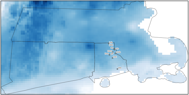
In the second script, we begin with reading in the modules and setting paths. I added an option at the top with a variable called temp_many_days; if it’s set to True, it will take the date range below it and retrieve temperatures for x to y days before the observation date in the point file. If it’s False, it will retrieve just the matching date. I also specify the names of columns in the input point observation shapefile that contain a unique ID number, name, and date. In this case the input data consists of ten sample points and dates that I’ve concocted, labeled alfa through juliett, all located in Rhode Island and stored as a shapefile.
import os,csv,rasterio
import matplotlib.pyplot as plt
import geopandas as gpd
from rasterio.plot import show
from datetime import datetime as dt
from datetime import timedelta
from datetime import date

#Calculate temps over multiple previous days from observation
temp_many_days=True # True or False
date_range=(1,7) # Range of past dates

#Inputs
point_file=os.path.join('input_points','test_obsv.shp')
raster_dir=os.path.join('input_raster','clipped')
outfolder='output'
if not os.path.exists(outfolder):
    os.makedirs(outfolder)

# Column names in point file that contain: unique ID, name, and date
obnum='OBS_NUM'
obname='OBS_NAME'
obdate='OBS_DATE'
Next, we loop through the folder of clipped raster files, and for each raster (ending in .tif) we grab the file name and extract the date from it. We take that date and store it in Python’s standard date format. The date becomes a key, and the path to the raster its value, which get added to a dictionary called rf_dict. For example, if we split the file name clipped_PRISM_tmean_stable_4kmD2_20200131_bil.tif using the underscores, counting from zero we get the date in the 5th position, 20200131. Converting that to the standard datetime format gives us datetime.date(2020, 1, 31).
rf_dict={} # Create dictionary of dates and raster file names

for rf in os.listdir(raster_dir):
    if rf.endswith('.tif'):
        rfdatestr=rf.split('_')[5]
        rfdate=dt.strptime(rfdatestr,'%Y%m%d').date() #format of dates is 20200131
        rfpath=os.path.join(raster_dir,rf)
        rf_dict[rfdate]=rfpath
    else:
        pass
Then we read the observation point shapefile into a geodataframe, create an empty result_list that will hold each of our extracted values, and construct the header row for the list. If we are grabbing temperatures for multiple days, we generate extra header values to add to that row.
#open point shapefile
point_data = gpd.read_file(point_file)

result_list=[]
result_list.append(['OBS_NUM','OBS_NAME','OBS_DATE','RASTER_ROW','RASTER_COL','RASTER_FILE','TEMP'])

if temp_many_days==True:
    for d in range(date_range[0],date_range[1]):
        tcol='TMINUS_'+str(d)
        result_list[0].append(tcol)
    result_list[0].append('TEMP_RANGE')
    result_list[0].append('AVG_TEMP')
    temp_ftype='multiday_'
else:
    temp_ftype='singleday_'
Now the preliminaries are out of the way, and processing can begin. This post and tutorial helped me to grasp the basics of the process. We loop through the point data in the geodataframe (we indicate point.data.index because these are dataframe records we’re looping through). We get the observation date for the point and store that it the standard Python date format. Then we take that date, compare it to the dictionary, and get the path to the corresponding temperature raster for that date. We open that raster with rasterio, isolate the x and y coordinate from the geometry of the point observation, and retrieve the corresponding row and column for that coordinate pair from the raster. Then we read the value that’s associated with the grid cell at those coordinates. We take some info from the observation points (the number, name, and date) and the raster data we’ve retrieved (the row, column, file name, and temperature from the raster) and add it to a list called record.
#Pull out and format the date, and use date to look up file
for idx in point_data.index:
    obs_date=dt.strptime(point_data[obdate][idx],'%m/%d/%Y').date() #format of dates is 1/31/2020
    obs_raster=rf_dict.get(obs_date)
    if obs_raster == None:
        print('No raster available for observation and date',
              point_data[obnum][idx],point_data[obdate][idx])
    #Open raster for matching date, overlay point coordinates, get cell location and value
    else:
        raster=rasterio.open(obs_raster)
        xcoord=point_data['geometry'][idx].x
        ycoord=point_data['geometry'][idx].y
        row, col = raster.index(xcoord,ycoord)
        tempval=raster.read(1)[row,col]
        rfile=os.path.split(obs_raster)[1]
        record=[point_data[obnum][idx],point_data[obname][idx],
                point_data[obdate][idx],row,col,rfile,tempval]
If we had specified that we wanted a single day (option near the top of the script), we’d skip down to the bottom of the next block, append the record to the main result_list, and continue iterating through the observation points. Else, if we wanted multiple dates, we enter into a sub-loop to get data from a range of previous dates. The datetime timedelta function allows us to do date subtraction; if we subtract 1 from the current date, we get the previous day. We loop through and get rasters and the temperature values for the points from each previous date in the range and append them to an old_temps list; we also build in a safety mechanism in case we don’t have a raster file for a particular date. Once we have all the dates, we do some calculations to get the average temperature and range for that entire period. We do this on a copy of old_temps called all_temps, where we delete null values and add the current observation date. Then we add the average and range to old_temps, and old_temps to our record list for this point observation, and when finished we append the observation record to our main result_list, and proceed to the next observation.
       # Optional block, if pulling past dates
        if temp_many_days==True:
            old_temps=[]
            for d in range(date_range[0],date_range[1]):
                past_date=obs_date-timedelta(days=d) # iterate through days, subtracting
                past_raster=rf_dict.get(past_date)
                if past_raster == None: # if no raster exists for that date
                    old_temps.append(None)
                else:
                    old_raster=rasterio.open(past_raster)
                    # Assumes rasters from previous dates are identical in structure to 1st date
                    past_temp=old_raster.read(1)[row,col]
                    old_temps.append(past_temp)
            # Calculate avg and range, must exclude None values and include obs day
            all_temps=[t for t in old_temps if t is not None]
            all_temps.append(tempval)
            temp_range=max(all_temps)-min(all_temps)
            avg_temp=sum(all_temps)/len(all_temps)
            old_temps.extend([temp_range,avg_temp])
            record.extend(old_temps)
            result_list.append(record)
        else: # if NOT doing many days, just append data for observation day
            result_list.append(record)
    if (idx+1)%200==0:
        print('Processed',idx+1,'records so far...')
Once the loop is complete, we plot the last point and raster to the screen just to check that it looks good, and we write the results out to a CSV.
#Plot the points over the final raster that was processed
fig, ax = plt.subplots(figsize=(12,12))
point_data.plot(ax=ax, color='black')
show(raster, ax=ax)

today=str(date.today()).replace('-','_')
outfile='temp_observations_'+temp_ftype+today+'.csv'
outpath=os.path.join(outfolder,outfile)

with open(outpath, 'w', newline='') as writefile:
    writer=csv.writer(writefile, quoting=csv.QUOTE_MINIMAL, delimiter=',')
    writer.writerows(result_list)

print('Done. {} observations in input file, {} records in results'.format(len(point_data),len(result_list)-1))

Results and Wrap-up
Visit the GitHub repo for full copies of the scripts, plus input and output data. In creating test observation points, I purposefully added some locations that had identical coordinates, identical dates, dates that varied by a single day, and dates for which there would be no corresponding raster file in the sample data if we went one week back in time. I looked up single dates for all point observations manually, and a sample of multi-day selections as well, and they matched the output of the script. The scripts ran quickly, and the overall process seemed intuitive to me; resetting the metadata for rasters after masking is the one part that wouldn’t have occurred to me, and took a little bit of time to figure out. This solution worked well for this case, and I would definitely apply geospatial Python to a problem like this again. An alternative would have been to use a spatial database like PostGIS; this would be an attractive option if we were working with a bigger dataset and processing time became an issue. The benefit of using this Python approach is that it’s easier to share the script and replicate the process without having to set up a database.









You must be logged in to post a comment.