In this post I demonstrate how export a list of variables from a STATA dta file to an Excel spreadsheet, and how to create a STATA do file by using Python to read in a list of variables from a spreadsheet; the do file will generate an extract of attributes and observations from a larger dta file. Gallup Analytics microdata serves as the example.
Gallup Analytics Microdata
Many academic libraries subscribe to an online database called Gallup Analytics, which lets users explore and download summary statistics from a number of on-going polls and surveys conducted by the Gallup Organization, such as the US Daily Tracker poll, World Poll, and SPSS polling series. As part of the package, subscribing institutions also receive microdata files for some of the surveys, in STATA and SPSS formats. These files contain the anonymized, individual responses to the surveys. The microdata is valuable to social science researchers who use the responses to conduct statistical analyses.
Microdata in STATA
Naturally, the microdata is copyrighted and licensed for non-commercial research purposes to members of the university or institution who are covered by the license agreement, and cannot be shared outside the institution. Another stipulation is that the files cannot be shared in their entirety, even for members of the licensed institution; researchers must request individual extracts of variables and observations to answer a specific research question. This poses a challenge for the data librarian, who somehow has to communicate to the researcher what’s available in the files and mediate the request. Option 1 is to share the codebooks (which are also copyrighted and can’t be publicly distributed) with the researcher and haggle back and forth via email to iron out the details of the request. Option 2 is to have a stand-alone computer set up in the library, where a researcher can come and generate their own extract from files stored on a secure, internal network. In both cases, the manual creation of the extract and the researcher’s lack of familiarity with the contents of the data makes for a tedious process.
My solution was to create spreadsheets that list all of the variables in each dataset, and have the researcher check the ones they want. I created a resource guide that advertises and describes the datasets, and provides secure links to the Gallup codebooks and these spreadsheets, which are stored on a Google Drive and are protected via university authentication. The researcher can then fill out a Google form (also linked to from that page), where they describe the nature of the request, select the specific dataset of interest, specify filters on observations (rows), and upload the spreadsheet of requested variables (columns). Then, I can read the spreadsheet variables into Python and generate a STATA do file (STATA scripts stored in plain text format), to create the desired extract which I can share with the researcher.
Create List of STATA Variables in Excel Spreadsheet
First, I created a standard set of STATA do files to output lists of all variables to a spreadsheet for the different data files. An example for the US Daily Tracker poll from pre-2018 is below. I was completely unfamiliar with STATA, but the online docs and forums taught me what I needed to pull this together.
Some commands are the same across all the do files. I use describe and then translate to create a simple text file that saves a summary from the screen that counts rows and columns. Describe gives a description of the data stored in memory, while replace is used to swap out existing variables with a new subset. Then, generate select_vars gives me codebook information about the dataset (select_vars is a variable name I created), which I sort using the name column. The export excel command is followed by the specific summary fields I wish to output; the position of the variable, data type, variable label, and the variable name itself.
* Create variable list for Gallup US Tracker Survey 2008-2017

local y = YEAR in 1

describe,short
summarize YEAR
translate @Results gallup_tracker_`y'_summary.txt, replace

describe, replace
generate select_vars = ""
sort name

export excel position name type varlab select_vars using gallup_tracker_`y'_vars.xlsx, firstrow(variables) replace
The variation for this particular US Daily Tracker dataset is that the files are packaged as one file per year. I load the first file for 2008, and the do file saves the YEAR attribute as a local variable, which allows me to include the year in the summary and excel output file names. I had to run this do file for each subsequent year up to 2017. This is not a big deal as I’ll never have to repeat the process on the old files, as new data will be released in separate, new files. Other datasets imposed different requirements; the GPSS survey is packaged in eleven separate files for different surveys, and the updates are cumulative (each file contains older data plus any updates – Gallup sends us updated files a few times each year). For the GPSS, I prompt the user for input to specify the survey file name, and overwrite the previous Excel file.
With the do file in hand, you open STATA and the data file you want to process, change the working directory from the default user folder to a better location for storing the output, open the do file, and it runs and creates the variable list spreadsheet.
List of variables in Excel generated from STATA file. Users check the variables they want in an extract in the select_vars column
Create a STATA Do File with Python and Excel
Once a researcher submits their Google form and their selected variable spreadsheet (placing an X in a dedicated column to indicate that they want to include a variable), I run the Python script below. I use the openpyxl module to read the Excel file. I have to modify the paths, spreadsheet file name, and an integer for the particular survey each time I run it. I use the os module to navigate up and down through folders to store outputs in specific places. If the researcher specifies in the Google form that they want to filter observations, for example records for specific states or age ranges, I have to add those manually but I commented out a few examples that I can copy and modify. One caveat is that you must filter using the coded variable and not its label (i.e. if a month value is coded as 2 and its label is February, I must reference the code and not the label). Reading in the requested columns is straightforward; the script identifies cells in the selection column (E) that have an X, then grabs the variable name from the adjacent column.
# -*- coding: utf-8 -*-
"""
Pull selected gallup variables from spreadsheet to create STATA Do File
Frank Donnelly / GIS and Data Librarian / Brown University
"""

import openpyxl as xl, os
from datetime import date

thedate=date.today().strftime("%m%d%Y")
surveys={1:'gallup_covid',2:'gallup_gpss',3:'gallup_tracker',4:'gallup_world'}

rpath=os.path.join('requests','test') # MODIFY BASED ON INPUT
select_file=os.path.join(rpath,'gallup_tracker_2017_vars_TEST.xlsx') #MODIFY BASED ON INPUT
survey_file=surveys[3] #MODIFY BASED ON INPUT

dofile=os.path.join(rpath,'{}_vars_{}.do'.format(survey_file,thedate))
dtafile=os.path.join(os.path.abspath(os.getcwd()),rpath,'{}_extract_{}.dta'.format(survey_file,thedate))


#MODIFY to filter by observations - DO NOT ERASE EXAMPLES - copy, then modify
obsfilter=None
# obsfilter=None
# obsfilter='keep if inlist(STATE_NAME,"CT","MA","ME","NH","RI","VT")'
# obsfilter='keep if inrange(WP1220,18,64)'
# obsfilter='keep if SC7==2 & MONTH > 6'
# obsfilter='keep if FIPS_CODE=="44007" | FIPS_CODE=="25025"'

workbook = xl.load_workbook(select_file)
ws = workbook['Sheet1']

# May need to modify ws col and cell values based on user input
vlist=[]
for cell in ws['E']:
    if cell.value in ('x','X'):
        vlist.append((ws.cell(row=cell.row, column=2).value))
outfile = open(dofile, "w")
outfile.writelines('keep ')
outfile.writelines(" ".join(vlist)+"\n")
if obsfilter==None:
    pass
else:
    outfile.writelines(obsfilter+"\n")
outfile.writelines('save '+dtafile+"\n")
outfile.close()
print('Created',dofile)
The plain text do file begins with the command keep followed by the columns, and if requested, an additional keep statement to filter by records. The final save command will direct the output to a specific location.
All that remains is to open the requested data file in STATA, open the do file, and an extract is created. Visit my GitHub for the do files, Python script, and sample output. The original source data and the variable spreadsheets are NOT included due to licensing issues; if you have the original data files you can generate what I’ve described here. Sorry, I can’t share the Gallup data with you (so please don’t ask). You’ll need to contact your own university or institution to determine if you have access.
I’ve suffered from a bit of the blues in this new year, so two weekends ago I logged into Steam and bought a new game to relax a little. It’s been a few years since I’ve bought a new game, and in playing this one and perusing my existing collection I realized they all had one thing in common: geography plays a central role in all of them. So in this first post of the year, I’ll explore the role of geography in video games using examples from my favorites.
Terrain and Exploration in 4X Games
My latest purchase is Signals by MKDB Studios, an indie husband and wife developer team in the UK. It can be classified as a “casual” game, in that it’s: easy to learn and play yet possesses subtle complexity, is relatively relaxing in that it doesn’t require constant action and mental exertion, and you can finish a scenario or round in an hour or so. In Signals, you are part of a team that has discovered an alien signaling device on a planet. The device isn’t working; fixing it requires setting up a fully functional research station adjacent to the device, so you can unlock its secrets. The researchers need access to certain key elements that you must discover and mine. The planet you’re on doesn’t have these resources, so you’ll need to explore neighboring systems in the sector and beyond to find and bring them back.
Space travel is expensive, and the further you journey the more credits (money) you’ll need. To fund travel to neighboring systems in search of the research components (lithium, silicon, and titanium) you can harvest and sell a variety of other resources including copper, iron, aluminum, salt, gold, gems, diamonds, oil, and plutonium. As you flood the market with resources their value declines, yielding diminishing returns. You must be strategic in hopping from planet to planet and deciding what to harvest and sell. Mining resources incurs initial fixed costs for building harvesters (one per resource patch), a solar array for powering them (which can only cover a small area), and a trade post for moving resources to the market (one per planet).
Terrain view on Signals. Harvesters extracting resources in the center, other resource patches to the right
The game has two distinct views: one displays the terrain of the planet you’re on, while the other is a map of the sector(s) with different solar systems, so you can explore the planets and their resources and make travel plans. Different terrain provides different resources and imposes limits on game play. You are precluded from constructing buildings on water and mountains, and must clear forests if you wish to build on forested spaces. Terrain varies by type of planet: habitable Earth-like, red Mars-like, ice worlds, and desert worlds. The type of world influences what you will find in terms of resources; salt is only found on habitable worlds, while iron is present in higher quantities on Mars-like worlds. Video games, like maps, are abstractions of reality. The planet view shows you just a small slice of terrain that stands in for the entire world, so that the game can emphasize the planet hopping concept that’s central to its design. The other view – the sector map – is used for navigation and reference, keeping track of where you are, where you’ve been, and where you should go next.
Select a system in the sector map……to view its planets and resources.
The use of terrain and the role of physical geography are key aspects in simulators (like SimCity, an old favorite) and the so-called 4X games which focus on exploration, mining, trading, and fighting, although not all games employ all four aspects (Signals has no fighting or conquest component). Another example of a 4X game is Factorio by Wube Software, which I’ve written about previously. Like Signals, exploring terrain and mining resources are central to the game play. Similarities end there, as Factorio is anything but a casual game. It requires a significant amount of research and experimentation to learn how to play, which means consulting wikis, tutorials, and YouTube. It also takes a long time – 30 to 40 hours to complete one game!
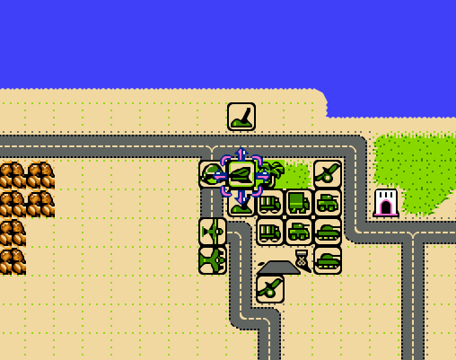
The action in Factorio occurs on a single planet, where you’re looking for resources to mine to build higher order goods in factories, that you turn into even higher order products as you unlock more technologies by conducting research, with the ultimate goal of constructing a rocket to get off the planet. There are also two map views: the primary terrain view that you navigate as the player, and an overview map displaying the extent of the planet that you’ve explored. You begin with good knowledge of what lies around you, as you captured this info before your spaceship crashed and marooned you here. Beyond that is simply unknown darkness. To reveal it, you physically have to go out and explore, or build radar devices that gradually expand your knowledge. The terrain imposes limits on building and movement; water can’t be traversed or built upon, canyons block your path, and forests slow movement and prevent construction unless you chop them down (or build elsewhere). The world generated in Factorio is endless, and as you use up resources you have to push outward to find more; you can build vehicles to travel more quickly, while conveyor belts and trains can transport resources and products to and around your factory; this growing logistical puzzle forms a large basis of the game.
Mining drills in Factorio extracting stone. Belts transport resources short distances, while trains cover longer distances.
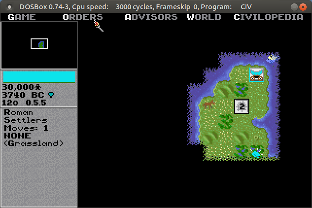
The role of terrain and exploration has long been a mainstay in these kinds of games. Thanks to DOSbox (an emulator that let’s you run DOS and DOS programs on any OS), I was recently playing the original Sid Meier’s Civilization from 1991 by Microprose. This game served as a model for many that followed. Your small band of settlers sets out in 4000 BC, to found the first city for your particular civilization. You can see the terrain immediately around you, but the rest of the world is shrouded in darkness. Moving about slowly reveals more of the world, and as you meet other civs you can exchange maps to expand your knowledge. The terrain – river basins, grasslands, deserts, hills, mountains, and tundra – influences how your cities will grow and develop based on the varying amount of food and resources it produces. Terrain also influences movement; it is tougher and takes longer to move over mountains versus plains, and if you construct roads that will increase speed and trade. The terrain also influences attack and defense capabilities for military units…
The unknown, unexplored world is shrouded in darkness in Civilization
Terrain and Exploration in Strategic Wargames
Strategic war games are another genre where physical geography matters. One weekend shortly after the pandemic lock-down began in 2020, I dug my old Nintendo out of the closet and replayed some of my old favorites. Desert Commander by Kemco was a particular favorite, and one of Nintendo’s only war strategy games. You command one of two opposing armies in the North African desert during World War II, and your objective is simple: eliminate the enemy’s headquarters unit, or their entire army. You have a mix of tanks, infantry, armored cars, artillery, anti-aircraft guns, supply trucks, fighters, and bombers at your command. Each unit varies in terms of range of movement and offensive and defensive strength, in total and relative to other units. Tanks are powerful attackers, but weak defenders against artillery and hopeless against bombers. Armored cars cruise quickly across the sands compared to slowly trudging infantry.
Terrain also influences movement, offense, and defense. You can speed along a road, but if you’re attacked by planes or enemy tanks you’ll be a sitting duck. Desert, grassland, wilds (mountains), and ocean make up the rest of the terrain, but scattered about are individual features like pillboxes and oases which provide extra defense. A novel aspect of the game was its reliance on supply: units run low on fuel and ammo, and after combat their numbers are depleted. You can supply fuel and ammo to ground units with trucks, but eventually these also run out of gas. Scattered about the map are towns, which are used for resupply and reinforcement. There are a few airfields scattered about, which perform the same functions for aircraft. Far from being a simple battle game, you have to constantly gauge your distance and access to these supply bases, and consider the terrain that you’re fighting on. The later scenarios leave you hopelessly outnumbered against the enemy, which makes the only winning strategy a defensive one where you position your headquarters and the bulk of your forces at the best strong point, while simultaneously sending out a smaller strike force to get the enemy HQ.
Units and terrain in NES Desert Commander. Towns and airfields are used for resupply.
There have been countless iterations and updates on this type of game. One that I have in my Steam library is Unity of Command by 2×2 Games, which pits the German and Soviet armies in the campaigns around Stalingrad during World War II. Like most modern turn-based games, the grid structure (used in Desert Commander) has been replaced with a hex structure, reflecting greater adjacency between areas. Again, there are a mix of different units with different strengths and capabilities. The landscape on the Russian steppe is flat, so much of the terrain challenge lies in securing bridgeheads or flanking rivers when possible, as attacking across them is suicidal. The primary goal is to capture key objectives like towns and bridgeheads in a given period of turns. A unit’s attack and movement phase are not strictly separated, so you can attack with a unit, move out of the way, and move another in to attack again until you defeat a given enemy. This opens up a hole, allowing you to pour more units through a gap to capture territory and move towards the objectives. The supply concept is even more crucial in UOC; as units move beyond their base, which radiates from either a single point or from a roadway, they will eventually run out of supplies and will be unable to fight. By pushing through gaps in defense and outflanking the enemy, you can capture terrain that cuts off this supply, which is more effective than trying to attack and destroy everything.
Unity of Command Stalingrad Campaign. Push units through gaps to capture objectives and cut off enemy supplies.
The most novel take on this type of game that I’ve seen is Radio General by Foolish Mortals. This WWII game is a mix of strategy and history lesson, as you command and learn about the Canadian army’s role in the war (it incorporates an extensive amount of real archival footage). As the general commanding the army, you can’t see the terrain, or even where any of the units are – including your own. You’re sitting behind the lines in a tent, looking at a topographic map and communicating with your army – by voice! – on the radio. You check in and confirm where they are, so you can issue orders (“Charlie company go to grid cell Echo 8”), and then slide their little unit icons on the map to their last reported position. They radio in updates, including the position of enemy units. The map doesn’t give you complete and absolute knowledge in this game; instead it’s a tool that you use to record and understand what’s going on. Another welcome addition is the importance of elevation, which aids or detracts in movement, attack, defense, and observation. A unit sitting on top of a hill can relay more information to you about battlefield circumstances compared to one hunkered down in a valley.
In Radio General, the topo map is the battlefield. You rely on the radio to figure out where your units, and the enemy units, are.
Strategy Games with the Map as Focal Point
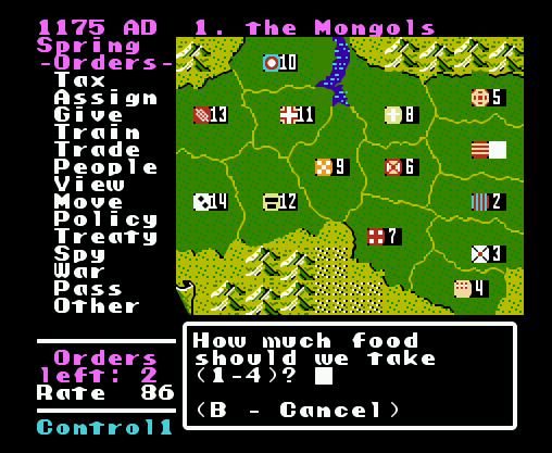
While terrain takes center stage in many games, in others all the action takes place on a map. Think of board games like Risk, where the map is the board and players capture set geographic areas like countries, which may be grouped into hierarchies (like continents) that yield more resources. Unlike the terrain-based games where the world is randomly generated, most map-based games are relatively fixed. Back to the Nintendo, the company Koei was a forerunner of historical strategy games on consoles, my favorite being Genghis Khan. The basic game view was the map, which displayed the “countries” of the world in the late 12th and early 13th centuries. Each country produced specialized resources based on its location, had military units unique to its culture, and produced gold, food, and resources based on its infrastructure. Your goal was to unite Mongolia and then conquer the world (of course). Once you captured other countries, they remained as distinct areas within your empire, and you would appoint governors to manage them. When invading, the view switched from an administrative map mode to a battlefield terrain mode, similar to ones discussed previously.
Genghis Khan on the original NES. The map is the focal point of the game.
Fast forward to now, and Paradox has become a leading developer of historical strategy games. Crusader Kings 2 is one of their titles that I have, where the goal is to rule a dynasty from the beginning to the end of the medieval period in the old world. Conquering the entire world is unlikely; you aim to rule some portion of it, with the intention of earning power and prestige for your dynasty through a variety of means, warlike and peaceful. These are complex games, which require diving into wikis and videos to understand all the medieval mechanics that you need to keep the dynasty going. Should you use gavelkind, primogeniture, seniority, or feudal elective succession? Choose wisely, otherwise your kingdom could fracture into pieces upon your demise, or worse your nefarious uncle could take the throne.
CK2 takes human geographical complexity to a new level with its intricate hierarchy of places. The fundamental administrative unit on the map is a county. Within the county you have sub-divisions, which in GIS-speak are like “points in polygons”: towns ruled by a non-noble mayor, parishes ruled by a bishop, and maybe a barony ruled by a noble baron. Ostensibly, these would be vassals to the count, while the count in turn is a vassal to a duke. Several counties form a duchy, which in turn make up a kingdom, and in some cases several kingdoms are part of empires (i.e. Holy Roman and Byzantine). In every instance, rulers at the top of the chain will hold titles to smaller areas. A king holds a title to the kingdom, plus one or more duchies, one or more counties (the king’s demesne), and maybe a barony or two. If he / she doesn’t hold these titles directly, they are granted to a vassal. A big part of the game is thwarting the power of vassals to lay claim to your titles, or if you are a vassal, getting claims to become the rightful heir. Tracking and shaping family relations and how they are tied to places is a key to success, more so than simply invading places.
Geographic hierarchy in Crusader Kings 2. Middlesex is a county with a town, barony, and parish. It’s one of four counties in the Duchy of Essex, in the Kingdom of England.
Which in CK2, is hard to do. Unlike other war games, you can’t invade whoever you want (unless they are members of a rival religion). The only way to go to war is if you have a legitimate claim to territory. You gain claims through marriage and inheritance, through your vassals and their claims, by fabricating claims, or by claiming an area that’s a dejure part of your territory, i.e. that is historically and culturally part of your lands. While the boundaries of the geographic units remain stable, their claims and dejure status change over time depending on how long they’re held, which makes for a map that’s dynamic. In another break from the norm, the map in CK2 performs all functions; it’s the main screen for game play, both administration and combat. You can modify the map to show terrain, political boundaries, and a variety of other themes.
Conclusion
I hope you enjoyed this little tour, which merely scratches the surface of the relation between geography and video games, based on a small selection of games I’ve played and enjoyed over the years. There’s a tight relationship between terrain and exploration, and how topography influences resource availability and development, the construction of buildings, movement, offense and defense. In some cases maps provide the larger context for tracking and explaining what happens at the terrain level, as well as navigating between different terrain spaces. In other cases the map is the central game space, and the terrain element is peripheral. Different strategies have been employed for equating the players knowledge with the map; the player can be all knowing and see the entire layout, or they must explore to reveal what lies beyond their immediate surroundings.
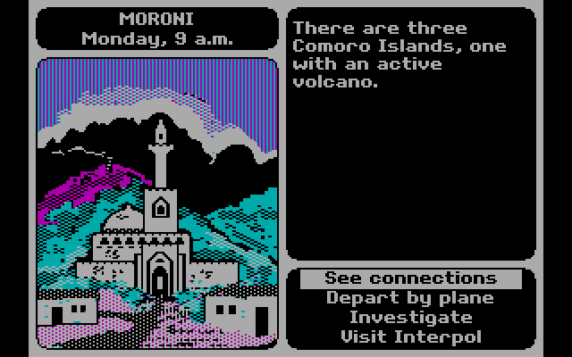
There are also a host of geographically-themed games that make little use of maps or terrain. For example, Mini Metro by Dinosaur Polo Club is a puzzle game where you connect constantly emerging stations to form train lines to move passengers, using a schematic resembling the London tube map. In this game, the connectivity between nodes in a network is what’s important, and you essentially create the map as you go. Or 3909 LLC’s Papers, Please, a dystopian 1980s “document simulator” where you are a border control guard in an authoritarian country in a time of revolution, checking the documentation of travelers against ever changing rules and regulations (do traveler’s from Kolechia need a work permit? Is Skal a city in Orbistan or is this passport a forgery…). Of course, we can’t end this discussion without mentioning Where in the World is Carmen Sandiego, Broderbund’s 1985 travel mystery that introduced geography and video games to many Gen Xers like myself. Without it, I may have never learned that perfume is the chief export of Comoros, or that Peru is slightly smaller than Alaska!
Where in the World is Carmen Sandiego? In hi-tech CGA resolution!
Even though I’ve left New York, there are still occasions where I refer back to NYC resources in order to help students and faculty here with NYC-based research. Most recently I’ve revisited NYC DOITT’s Geoclient API for geocoding addresses, and I discovered a number of things have changed since I’ve last used it a few years ago. I’ll walk through my latest geocoding script in this post.
First and foremost: if you landed on this page because you’re trying to figure out how to get your Geoclient API key to work, the answer is:
&subscription-key=YOURKEYHERE
This replaces the old format that required you to pass an app id and key. I searched through two websites and scanned through hundreds of pages of documentation, only to find this solution in a cached Google search result, as the new docs don’t mention this change and the old docs still have the previous information and examples of the application ID and key. So – hopefully this should save you some hours of frustration.
I was working with someone who needed to geocode a subset of the city’s traffic violation data from the open data portal, as the data lacks coordinates. It’s also missing postal city names and ZIP Codes, which precludes using most geocoders that rely on this information. Even if we had these fields, I’ve found that many geocoders struggle with the hyphenated addresses used throughout Queens, and some work-around is needed to get matches. NYC’s geoclient is naturally able to handle those Queens addresses, and can use the borough name or code for locating addresses in lieu of ZIP Codes. The traffic data uses pseudo-county codes, but it’s easy to replace those with the corresponding borough codes.
The older documentation is still solid for illustrating the different APIs and the variables that are returned; you can search for a parsed or non-parsed street address, street intersections, places of interest or landmarks, parcel blocks and lots, and a few others.
I wrote some Python code that I’ve pasted below for geocoding addresses that have house numbers, street, and borough stored in separate fields using the address API, and if the house number is missing we try again by doing an intersection search, as an intersecting street is stored in a separate field in the traffic data. In the past I used a thin client for accessing the API, but I’m skipping that as it’s simpler to just build the URLs directly with the requests module.
The top of the script has the standard stuff: the name of the input file, the column locations (counting from zero) in the input file that contain each of the four address components, the base URL for the API, a time function for progress updates, reading the API key in from a file, and looping through the input CSV with the addressees to save the header row in one list and the records in a nested list. I created a list of fields that are returned from the API that I want to hold on to and add them to the header row, along with a final variable that records the results of the match. In addition to longitude and latitude you can also get xCoordinate and yCoordinate, which are in the NY State Plane Long Island (ft-US) map projection. I added a counts dictionary to keep track of the result of each match attempt.
Then we begin a long loop – this is a bit messy and if I had more time I’d collapse much of this into a series of functions, as there is repetitive code. I loop through the index and value of each record beginning with the first one. The loop is in a try / except block, so in the event that something goes awry it should exit cleanly and write out the data that was captured. We take the base url and append the address request, slicing the record to get the values for house, street, and borough into the URL. An example of a URL after passing address components in:
https://api.nyc.gov/geo/geoclient/v1/address.json?houseNumber=12345&street=CONEY ISLAND AVE&borough=BROOKLYN&subscription-key=KEYGOESHERE
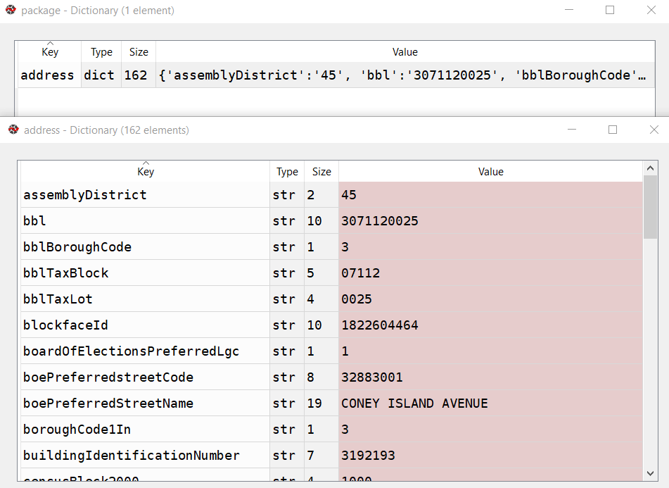
Pass that URL to the requests module and get a response back. If an address is returned, the JSON resembles a Python dictionary, with ‘address’ as the key and the value as another dictionary with key value pairs of several variables. Otherwise, we get an error message that something was wrong with the request.
A successful address match returns an address dictionary, with a sub-dictionary of keys and values
The loop logic:
If the package contains an ‘address’ key, flatten to get the sub-dictionary
If ‘longitude’ is present as a key, a match is returned, get the relevant fields and append to the record
Else if the dictionary contains a ‘message’ key with a value that the house number was missing, do an intersection match
If the package contains an ‘intersection’ key, flatten to get the sub-dictionary
If ‘longitude’ is present as a key, a match is returned, get the relevant fields and append to the record
If not, there was no intersection match, just get the messages and append blanks for each value to the record
If not, an error was returned, capture the error and append blanks for each value to the record, and continue
If not, there was no address match, just get the messages and append blanks for each value to the record
If not, an error was returned, capture the error and append blanks for each value to the record, and continue
The API has limits of 2500 matches per minute and 500k per day, so after 2000 records I built in a pause of 15 seconds. Once the process finishes, successfully or not, the records are written out to a CSV file, header row first followed by the records. If the process bailed prematurely, the last record and its index are printed to the screen. This allows you to rerun the script where you left off, by changing the start index in the variables list at the top of the script from 0 to the last record that was read. When it comes time to write output, the previous file is appended rather than overwritten and the header row isn’t written again.
It took about 90 minutes to match a file of 25,000 records. I’d occasionally get an error message that the API key was bad for a given record; the error would be recorded and the script continued. It’s likely that there are illegal characters in the input fields for the address that end up creating a URL where the key parameter can’t be properly interpreted. I thought the results were pretty good; beyond streets it was able to recognize landmarks like large parks and return matched coordinates with relevant error messages (example below). Most of the flops were, not surprisingly, due to missing borough codes or house numbers.
Output fields from the NYC Geoclient written to CSV
To use this code you’ll need to sign up for an NYC Developer API account, and then you can request a key for the NYC Geoclient service. Store the key in a text file in the same folder as the script. I’m also storing inputs and outputs in the same folder, but with a few functions from the os module you can manipulate paths and change directories. If I get time over the winter break I may try rewriting to incorporate this, plus functions to simplify the loops. An alternative to the API would be to download the LION street network geodatabase, and you could set up a local address locator in ArcGIS Pro. Might be worth doing if you had tons of matches to do. I quickly got frustrated with with the ArcGIS documentation and after a number of failed attempts I opted to use the Geoclient instead.
"""
Match addresses to NYC Geoclient using house number, street name, and borough
Frank Donnelly / GIS and Data Librarian / Brown University
11/22/2021 - Python 3.7
"""

import requests, csv, time

#Variables
addfile='parking_nov2021_nyc.csv' #Input file with addresses
matchedfile=addfile[:-4]+'_output.csv' #Output file with matched data
keyfile='nycgeo_key.txt' #File with API key
start_idx=0 #If program breaks, change this to pick up with record where you left off
#Counting from 0, positions in the CSV that contain the address info
hous_idx=23
st_idx=24
boro_idx=21
inter_idx=25
base_url='https://api.nyc.gov/geo/geoclient/v1/'

def get_time():
    time_now = time.localtime() # get struct_time
    pretty_time = time.strftime("%m/%d/%Y, %H:%M:%S", time_now)
    return pretty_time

print('*** Process launched at', get_time())

#Read api key in from file
with open(keyfile) as key:
    api_key=key.read().strip()

records=[]

with open(addfile,'r') as infile:
    reader = csv.reader(infile)
    header = next(reader) # Capture column names as separate list
    for row in reader:
        records.append(row)

# Fields returned by the API to capture
# https://maps.nyc.gov/geoclient/v1/doc
fields=['message','message2','houseNumber','firstStreetNameNormalized',
        'uspsPreferredCityName','zipCode','longitude','latitude','xCoordinate',
        'yCoordinate']
header.extend(fields)
header.append('match_result')
datavals=len(fields)-2 # Number of fields that are not messages
counts={'address match':0, 'intersection match':0,
        'failed address':0, 'failed intersection':0,
        'error':0}

print('Finished reading data from', addfile)
print('*** Geocoding process launched at',get_time())

for i,v in enumerate(records[start_idx:]):
    try:
        data_url = f'{base_url}address.json?houseNumber={v[hous_idx]}&street={v[st_idx]}&borough={v[boro_idx]}&subscription-key={api_key}'
        response=requests.get(data_url)
        package=response.json()
        # If an address is returned, continue
        if 'address' in package:
            result=package['address']
            # If longitude is returned, grab data
            if 'longitude' in result:
                for f in fields:
                    item=result.get(f,'')
                    v.append(item)
                v.append('address match')
                counts['address match']=counts['address match']+1
            # If there was no house number, try street intersection match instead
            elif 'message' in result and result['message']=='INPUT CONTAINS NO ADDRESS NUMBER' and v[inter_idx] not in ('',None):
                try:
                    data_url = f'{base_url}intersection.json?crossStreetOne={v[st_idx]}&crossStreetTwo={v[inter_idx]}&borough={v[boro_idx]}&subscription-key={api_key}'
                    response=requests.get(data_url)
                    package=response.json()
                    # If an intersection is returned, continue
                    if 'intersection' in package:
                        result=package['intersection']
                        # If longitude is returned, grab data
                        if 'longitude' in result:
                            for f in fields:
                                item=result.get(f,'')
                                v.append(item)
                            v.append('intersection match')
                            counts['intersection match']=counts['intersection match']+1
                        # Intersection match fails, append messages and blank values
                        else:
                            v.append(result.get('message',''))
                            v.append(result.get('message2',''))
                            v.extend(['']*datavals)
                            v.append('failed intersection')
                            counts['failed intersection']=counts['failed intersection']+1
                    # Error returned instead of intersection
                    else:
                        v.append(package.get('message',''))
                        v.append(package.get('message2',''))
                        v.extend(['']*datavals)
                        v.append('error')
                        counts['error']=counts['error']+1
                        print(package.get('message',''))
                        print('Geocoder error at record',i,'continuing the matching process...')
                except Exception as e:
                     print(str(e))
            # Address match fails, append messages and blank values
            else:
                v.append(result.get('message',''))
                v.append(result.get('message2',''))
                v.extend(['']*datavals)
                v.append('failed address')
                counts['failed address']=counts['failed address']+1
        # Error is returned instead of address
        else:
            v.append(package.get('message',''))
            v.append(package.get('message2',''))
            v.extend(['']*datavals)
            v.append('error')
            counts['error']=counts['error']+1
            print(package.get('message',''))
            print('Geocoder error at record',i,'continuing the matching process...')
        if i%2000==0:
            print('Processed',i,'records so far...')
            time.sleep(15)
    except Exception as e:
        print(str(e))

# First attempt, write to new file, but if break happened, append to existing file
if start_idx==0:
    wtype='w'
else:
    wtype='a'

end_idx=start_idx+i

with open(matchedfile,wtype,newline='') as outfile:
    writer = csv.writer(outfile, delimiter=',', quotechar='"',
                        quoting=csv.QUOTE_MINIMAL)
    if wtype=='w':
        writer.writerow(header)
        writer.writerows(records[start_idx:end_idx])
    else:
        writer.writerows(records[start_idx:end_idx])
print('Wrote',i+1,'records to file',matchedfile)
print('Final record written was number',i,':\n',v)
for k,val in counts.items():
    print(k,val)
print('*** Process finished at',get_time())
In late summer and early fall I was hammering out the draft for an ALA Tech Report on using census data for research (slated for release early 2022). The earliest 2020 census figures have been released and there are several issues surrounding this, so I’ll provide a summary of what’s happening here. Throughout this post I link to Census Bureau data sources, news bulletins, and summaries of trends, as well as analysis on population trends from Bill Frey at Brookings and reporting from Hansi Lo Wang and his colleagues at NPR.
Count Result and Reapportionment Numbers
The re-apportionment results were released back in April 2020, which provided the population totals for the US and each of the states that are used to reallocate seats in Congress. This data is typically released at the end of December of the census year, but the COVID-19 pandemic and political interference in census operations disrupted the count and pushed all the deadlines back.
Despite these disruptions, the good news is that the self-response rate, which is the percentage of households who submit the form on their own without any prompting from the Census Bureau, was 67%, which is on par with the 2010 census. This was the first decennial census where the form could be submitted online, and of the self-responders 80% chose to submit via the internet as opposed to paper or telephone. Ultimately, the Bureau said it reached over 99% of all addresses in its master address file through self-response and non-response follow-ups.
The bad news is that the rate of non-response to individual questions was much higher in 2020 than in 2010. Non-responses ranged from a low of 0.52% for the total population count to a high of 5.95% for age or date of birth. This means that a higher percentage of data will have to be imputed, but this time around the Bureau will rely more on administrative records to fill the gaps. They have transparently posted all of the data about non-response for researchers to scrutinize.
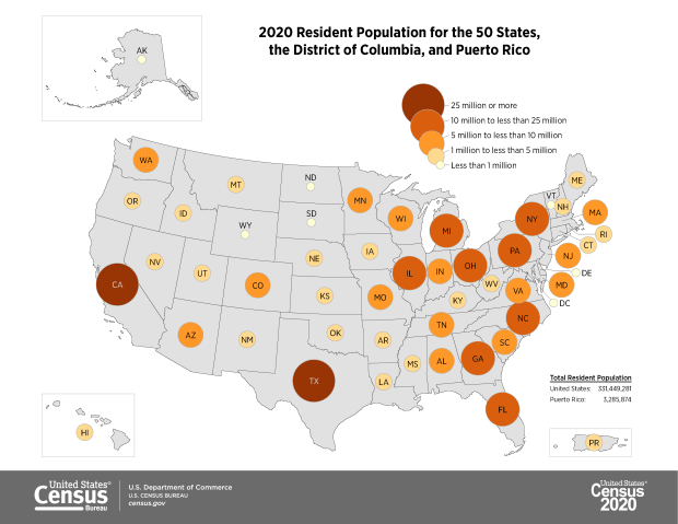
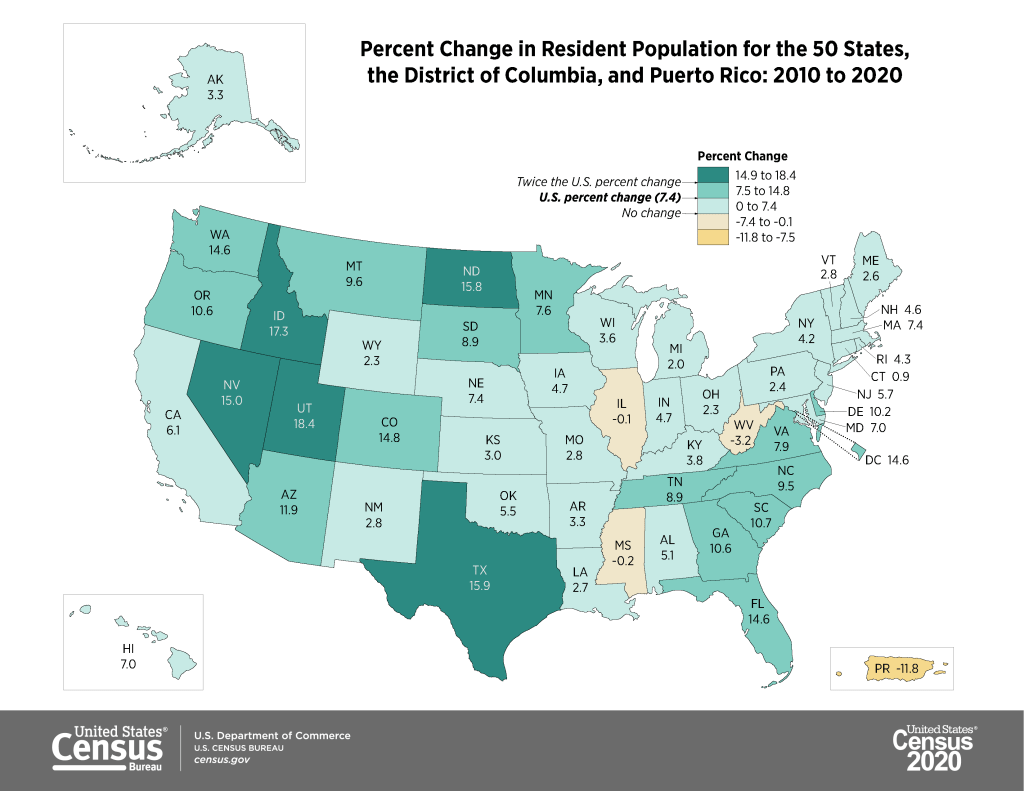
The apportionment results showed that the population of the US grew from approximately 309 million in 2010 to 331 million in 2020, a growth rate of 7.35%. This is the lowest rate of population growth since the 1940 census that followed the Great Depression. Three states lost population (West Virginia, Mississippi, and Illinois), which is the highest number since the 1980 census. The US territory of Puerto Rico lost almost twelve percent of its population. Population growth continues to be stronger in the West and South relative to the Northeast and Midwest, and the fastest growing states are in the Mountain West.
The first detailed population statistics were released as part of the redistricting data file, PL 94-171. Data in this series is published down to the block level, the smallest geography available, so that states can redraw congressional and other voting districts based on population change. Normally released at the end of March, this data was released in August 2021. This is a small package that contains the following six tables:
P1. Race (includes total population count)
P2. Hispanic or Latino, and Not Hispanic or Latino by Race
P3. Race for the Population 18 Years and Over
P4. Hispanic or Latino, and Not Hispanic or Latino by Race for the Population 18 Years and Over
P5. Group Quarters Population by Major Group Quarters Type
H1. Occupancy Status (includes total housing units)
The raw data files for each state can be downloaded from the 2020 PL 94-171 page and loaded into stats packages or databases. That page also provides infographics (including the maps embedded in this post) and data summaries. Data tables can be readily accessed via data.census.gov, or via IPUMS NHGIS.
The redistricting files illustrate the increasing diversity of the United States. The number of people identifying as two or more races has grown from 2.9% of the total population in 2010 to 10.2% in 2020. Hispanics and Latinos continue to be the fastest growing population group, followed by Asians. The White population actually shrank for the first time in the nation’s history, but as NPR reporter Hansi-Lo Wang and his colleagues illustrate this interpretation depends on how one measures race; as race alone (people of a single race) or persons of any race (who selected white and another race), and whether or not Hispanic-whites are included with non-Hispanic whites (as Hispanic / Latino is not a race, but is counted separately as an ethnicity, and most Hispanics identify their race as White or Other). The Census Bureau has also provided summaries using the different definitions. Other findings: the nation is becoming progressively older, and urban areas outpaced rural ones in population growth. Half of the counties in the US lost population between 2010 and 2020, mostly in rural areas.
2020 Demographic and Housing Characteristics and the ACS
There still isn’t a published timeline for the release of the full results in the Demographic and Housing Characteristics File (DHC – known as Summary File 1 in previous censuses, I’m not sure if the DHC moniker is replacing the SF1 title or not). There are hints that this file is going to be much smaller in terms of the number of tables, and more limited in geographic detail compared to the 2010 census. Over the past few years there’s been a lot of discussion about the new differential privacy mechanisms, which will be used to inject noise into the data. The Census Bureau deemed this necessary for protecting people’s privacy, as increased computing power and access to third party datasets have made it possible to reverse engineer the summary census data to generate information on individuals.
What has not been as widely discussed is that many tables will simply not be published, or will only be summarized down to the county-level, also for the purpose of protecting privacy. The Census Bureau has invited the public to provide feedback on the new products and has published a spreadsheet crosswalking products from 2010 and 2020. IPUMS also released a preliminary list of tables that could be cut or reduced in specificity (derived from the crosswalk), which I’m republishing at the bottom of this post. This is still preliminary, but if all these changes are made it would drastically reduce the scope and specificity of the decennial census.
And then… there is the 2020 American Community Survey. Due to COVID-19 the response rates to the ACS were one-third lower than normal. As such, the sample is not large or reliable enough to publish the 1-year estimate data, which is typically released in September. Instead, the Census will publish a smaller series of experimental tables for a more limited range of geographies at the end of November 2021. There is still no news regarding what will happen with the 5-year estimate series that is typically released in December.
Needless to say, there’s no shortage of uncertainty regarding census data in 2020.
Tables in 2010 Summary File 1 that Would Have Less Geographic Detail in 2020(Proposed)
Table Name
Proposed 2020 Lowest Level of Geography
2010 Lowest Level of Geography
Hispanic or Latino Origin of Householder by Race of Householder
County
Block
Household Size by Household Type by Presence of Own Children
County
Block
Household Type by Age of Householder
County
Block
Households by Presence of People 60 Years and Over by Household Type
County
Block
Households by Presence of People 60 Years and Over, Household Size, and Household Type
County
Block
Households by Presence of People 75 Years and Over, Household Size, and Household Type
County
Block
Household Type by Household Size
County
Block
Household Type by Household Size by Race of Householder
County
Block
Relationship by Age for the Population Under 18 Years
County
Block
Household Type by Relationship for the Population 65 Years and Over
County
Block
Household Type by Relationship for the Population 65 Years and Over by Race
County
Block
Family Type by Presence and Age of Own Children
County
Block
Family Type by Presence and Age of Own Children by Race of Householder
County
Block
Age of Grandchildren Under 18 Years Living with A Grandparent Householder
County
Block
Household Type by Relationship by Race
County
Block
Average Household Size by Age
To be determined
Block
Household Type for the Population in Households
To be determined
Block
Household Type by Relationship for the Population Under 18 Years
To be determined
Block
Population in Families by Age
To be determined
Block
Average Family Size by Age
To be determined
Block
Family Type and Age for Own Children Under 18 Years
To be determined
Block
Total Population in Occupied Housing Units by Tenure
To be determined
Block
Average Household Size of Occupied Housing Units by Tenure
To be determined
Block
Sex by Age for the Population in Households
County
Tract
Sex by Age for the Population in Households by Race
County
Tract
Presence of Multigenerational Households
County
Tract
Presence of Multigenerational Households by Race of Householder
County
Tract
Coupled Households by Type
County
Tract
Nonfamily Households by Sex of Householder by Living Alone by Age of Householder
County
Tract
Group Quarters Population by Sex by Age by Group Quarters Type
State
Tract
Tables in 2010 Summary File 1 That Would Be Eliminated in 2020(Proposed)
Population in Households by Age by Race of Householder
Average Household Size by Age by Race of Householder
Households by Age of Householder by Household Type by Presence of Related Children
Households by Presence of Nonrelatives
Household Type by Relationship for the Population Under 18 Years by Race
Household Type for the Population Under 18 Years in Households (Excluding Householders, Spouses, and Unmarried Partners)
Families*
Families by Race of Householder*
Population in Families by Age by Race of Householder
Average Family Size by Age by Race of Householder
Family Type by Presence and Age of Related Children
Family Type by Presence and Age of Related Children by Race of Householder
Group Quarters Population by Major Group Quarters Type*
Population Substituted
Allocation of Population Items
Allocation of Race
Allocation of Hispanic or Latino Origin
Allocation of Sex
Allocation of Age
Allocation of Relationship
Allocation of Population Items for the Population in Group Quarters
American Indian and Alaska Native Alone with One Tribe Reported for Selected Tribes
American Indian and Alaska Native Alone with One or More Tribes Reported for Selected Tribes
American Indian and Alaska Native Alone or in Combination with One or More Other Races and with One or More Tribes Reported for Selected Tribes
American Indian and Alaska Native Alone or in Combination with One or More Other Races
Asian Alone with One Asian Category for Selected Groups
Asian Alone with One or More Asian Categories for Selected Groups
Asian Alone or in Combination with One or More Other Races, and with One or More Asian Categories for Selected Groups
Native Hawaiian and Other Pacific Islander Alone with One Native Hawaiian and Other Pacific Islander Category for Selected Groups
Native Hawaiian and Other Pacific Islander Alone with One or More Native Hawaiian and Other Pacific Islander Categories for Selected Groups
Native Hawaiian and Other Pacific Islander Alone or in Combination with One or More Races, and with One or More Native Hawaiian and Other Pacific Islander Categories for Selected Groups
Hispanic or Latino by Specific Origin
Sex by Single Year of Age by Race
Household Type by Number of Children Under 18 (Excluding Householders, Spouses, and Unmarried Partners)
Presence of Unmarried Partner of Householder by Household Type for the Population Under 18 Years in Households (Excluding Householders, Spouses, and Unmarried Partners)
Nonrelatives by Household Type
Nonrelatives by Household Type by Race
Group Quarters Population by Major Group Quarters Type by Race
Group Quarters Population by Sex by Major Group Quarters Type for the Population 18 Years and Over by Race
Total Races Tallied for Householders
Hispanic or Latino Origin of Householders by Total Races Tallied
Total Population in Occupied Housing Units by Tenure by Race of Householder
Average Household Size of Occupied Housing Units by Tenure
Average Household Size of Occupied Housing Units by Tenure by Race of Householder
Occupied Housing Units Substituted
Allocation of Vacancy Status
Allocation of Tenure
Tenure by Presence and Age of Related Children
* Counts for these tables are available in other proposed DHC tables. For example, the count of families is available in the Household Type table, which will be available at the block level in the 2020 DHC.
Upon receiving a reminder from WordPress that it’s time to renew my subscription, I looked back and realized I’ve been pretty consistent over the years. Since rebooting this blog in Sept 2017, with few exceptions I’ve fulfilled my goal to write one post per month.
Unfortunately, due to professional and personal constraints I’m going to have to break my streak and put posting on pause for a while. Hopefully I can return to writing in the fall. Until then, enjoy the rest of summer.
I just released a new edition of my introductory QGIS manual for QGIS 3.16 Hannover (the current long term release), and as always I’m providing it under Creative Commons for classroom use and self-directed learning. I’ve also updated my QGIS FAQs handout, which is useful for new folks as a quick reference. This material will eventually move to a Brown University website, but when that happens I’ll still hold on to my page and will link to the new spot. I’m also leaving the previous version of the tutorial written for QGIS 3.10 A Coruna up alongside it, but will pull that down when the fall semester begins.
The new edition has a new title. When I first wrote Introduction to GIS Using Open Source Software, free and open source (FOSS) GIS was a novelty in higher ed. QGIS was a lot simpler, and I had to pull in several different tools to accomplish basic tasks like CRS transformations and calculating natural breaks. Ten years later, many university libraries and labs with GIS services either reference or support QGIS, and the package is infinitely more robust. So a name change to simply Introduction to GIS with QGIS seemed overdue.
My move from Baruch CUNY to Brown prompted me to make several revisions in this version. The biggest change was swapping the NYC-based business site selection example with a Rhode Island-based public policy one in chapters 2 and 3. The goal of the new hypothetical example is to identify public libraries in RI that meet certain criteria that would qualify them to receive funding for after school programs for K-12 public school students (replacing the example of finding an optimal location for a new coffee shop in NYC). In rethinking the examples I endeavored to introduce the same core concepts: attribute table joins, plotting coordinates, and geoprocessing. In this version I do a better job of illustrating and differentiating between creating subsets of features by: selecting by attributes and location, filtering (a new addition), and deleting features. I also managed to add spatial joins and calculated fields to the mix.
Changes to chapter 4 (coordinate reference systems and thematic mapping) were modest; I swapped out the 2016 voter participation data with 2020 data. I slimmed down Chapter 5 on data sources and tutorials, but added an appendix that lists web mapping services that you can add as base maps. Some material was shuffled between chapters, and all in all I cut seven pages from the document to slim it down a bit.
As always, there were minor modifications to be made due to changes between software versions. There were two significant changes. First, QGIS no longer supports 32 bit operating systems for Windows; it’s 64 bit or nothing, but that seems to be fairly common these days. Second, the Windows installer file is much bigger (and thus slower to download), but it helps insure that all dependencies are there. Otherwise, the differences between 3.16 and 3.10 are not that great, at least for the basic material I cover. In the past there was occasionally a lack of consistency regarding basic features and terminology that you’d think would be well settled, but thankfully things are pretty stable this time around.
If you have any feedback or spot errors feel free to let me know. I imagine I’ll be treading this ground again after the next long term release take’s 3.16’s place in Feb / Mar 2022. For the sake of stability I always stick with the long term release and forego the latest ones; if you’re going to use this tutorial I’d recommend downloading the LTR version and not the latest one.


You must be logged in to post a comment.