I’m often asked about what the best approaches are for comparing US census data over time, to account for changes in census geography and to limit the amount of data processing you have to do in stitching data from different census years together. Census geography changes significantly each decade, and by and large the Census Bureau does not compile and publish historical comparison tables.

My primary suggestion is to use the National Historical Geographic Information System or NHGIS (I’ll mention some additional suggestions at the end of this post). Maintained by IPUMS at the University of Minnesota, NHGIS is the repository for all historic US census summary data from 1790 to present. While most of the data in the archive is published nominally (the format and structure in which the data was originally published), they do publish a set of Time Series Tables that compile multiple years of census data in one table. These tables come in two formats:

• Nominal tables: the data is published “as is”, based on the boundaries that existed at each point in time. If a geography was added or dropped over the course of the years, it falls in or out of the table in the given year that the change occurred. With a few exceptions, the earliest nominal tables begin with the 1970 census and are published for eight geographies: nation, regions, divisions, states, counties, census tracts, county subdivisions, and places.
• Standardized tables: the data has been normalized, where a geography for a single time period serves as the basis for all data in the table. The NHGIS is currently using 2010 as the basis, so that data prior and subsequent to 2010 has been modified to fit within the 2010 boundaries. This is achieved by aggregating block or block group data from each period to fit within the 2010 boundaries, and apportioning the data in cases where a block or group is split by a boundary. The earliest standardized tables begin with the 1990 census, and cover the basic 100% count data. Data is published for ten geographies: states, counties, census tracts, block groups, county subdivisions, places, congressional districts (as defined for the 110th-112th Congresses, 2007-2013), core based statistical areas (using 2009 metro area definitions), urban areas, and ZIP Code Tabulation Areas (ZCTAs).

Included in the documentation is a full list of time series tables, and whether they are available in nominal or standardized format. The availability of specific time periods and geographies varies. As of late 2024, the availability of standardized tables that include the 2020 census is currently limited to what was published in the early Public Redistricting Files. This will likely change in the near future to include additional 2020 data, and it’s possible that the standardized geography will eventually switch from 2010 to 2020 geography.

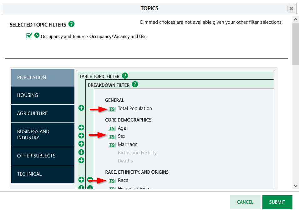
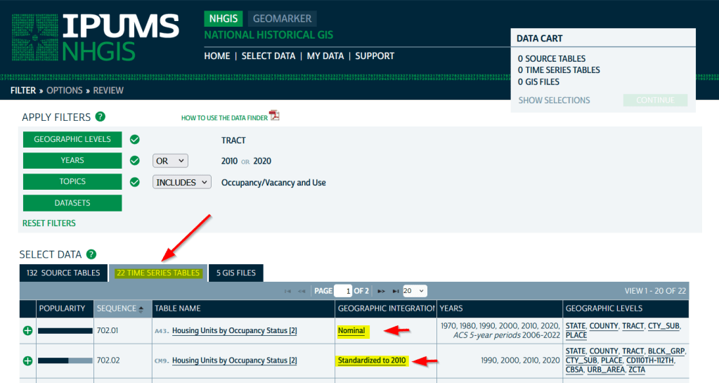
To access the Time Series Tables, you can browse the NHGIS without an account but you’ll need to create one in order to download anything. Once you launch NHGIS click on the Topics filter. In the list of topics, any topic under the Population or Housing category that has a “TS” flag next to it has at least one time series table. In the example below, I’ve used the filters to select census tracts for Geographic Level, 2010 and 2020 for Years, and Housing – Occupancy and Vacancy status as my Topic.

In the results at the bottom, the original Source Tables from each census are shown in the first tab. The Time Series Tables can be viewed by selecting the adjacent tab. The first two tables in this example are Housing Units by Occupancy Status. Clicking on the name of the tables reveals the variables that are included, and the source for the statistics. The first table is a nominal one that stretches from 1970 to the most recent ACS. The second table is a standardized one that covers 1990 to 2020. I’ve checked both boxes to add these to my cart.

The third tab in the results are GIS Files. If we want to map standardized data, we would choose just the boundaries for the standardized year, as all of the data in the table has been modified to fit these boundaries. If we were mapping nominal data, we would need to download boundary files for each time period and map them separately (unless they were stable geographies like states that haven’t changed since 1970).

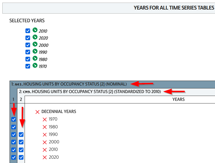
We hit the Continue button in the Cart panel when we’re ready to download. By default the extract will only include years and geographies we have filtered for. To add additional years or geos we can add them on this next screen. I’ve modified my list to get all available decennial years for each table. Note that if you’re going to select 5-year ACS data for nominal tables, choose only a few non-overlapping periods. In most cases you can’t filter geographies (i.e. select tracts within a state), you have to take them all. On the final screen you choose your structure; CSV is usually best, as is Time varies by column. Once you submit your request you’ll be prompted to log in if you haven’t already done so. Wait a bit for the extract to compile, then you can download the table and codebook.

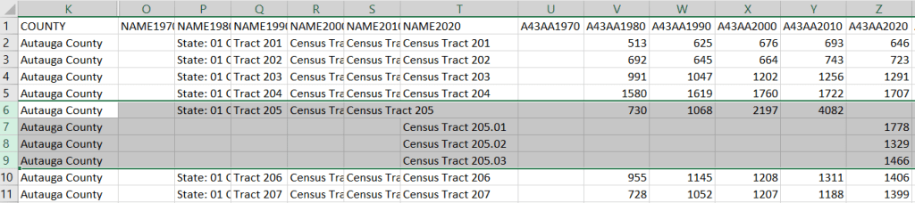
A portion of the nominal table is depicted below. This table includes identifiers and labels for each of the census years. The variables follow, ordered by variable and then by year. In this example, occupied housing units from 1970 to 2020 appear in the first block, and vacant units in the second. All the 1970 census tract values for Autauga County, Alabama are blank (as many rural counties in 1970 were un-tracted). We can see that values for census tract 205 run only from 1980 to 2010, with no value for 2020. The tract was split into three parts in 2020, and we see values for tracts 205.01, .02, and .03 appear in 2020. So in the nominal tables, geographies appear and disappear as they are created or destroyed. However, if geographic boundaries change but the name and designation for the geography do not, that geography persists throughout the time series in spite of the change.

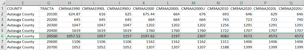
A portion of the standardized table is below. This table only includes identifiers and labels for the 2010 census, as all data was modified to fit the tract geography of that year. The values for each census year except 2010 are published in triplicate: an estimate, and a lower and upper bound for the estimate. If the values in these three columns differ, it indicates that a block (or block group) was split and reapportioned to fit within the tract boundary for 2010 (you may also see decimals, indicating a split occurred). You’d use the estimate in your work, while the bounds provide some indication of the estimate’s accuracy. Note in this table, tract 205 in Autauga County persists from 1990 to 2020, as it existed in 2010. Data from the three 2020 tracts was aggregated to fit the 2010 boundary.

The crosswalk tables that IPUMS used to create the standardized data are available, if you wanted or needed to generate your own normalized data. The best approach is to proceed from the bottom up, aggregating blocks to reformulate the data to the geography you wish to use. Some decennial census data, and all data from the ACS, is not available at the block level, which necessitates using block groups instead.

There are some alternatives for obtaining or creating time series census data, which could fit the bill depending on your use case (esp if you are looking at larger geographies). There’s also reference material that can help you make sense of changes.

1. The Longitudinal Tract Database at Brown University provides tract-level crosswalks from 1970 to 2020. They also provide some pre-compiled data tables generated from the crosswalk.
2. For short term comparisons, the ACS includes Comparison Profile Tables for states, counties, places, and metro areas that compare two non-overlapping time periods. For example, here is the 5-year ACS Comparative Demographic Estimates profile for Providence RI in 2022 (compares 2018-2022 with 2013-2017).
3. Use an interactive mapping tool like the Social Explorer to make side by side comparison maps from two time periods. They also incorporate some of the NHGIS standardized data into their database. (SE is a subscription-based product; if you’re at a university see if your library subscribes).
4. The Population and Housing Unit Estimates program publishes annual estimates for states, counties, and metro areas in decade by decade spreadsheets. The MCDC has created some easy to use tools for summarizing and charting this data to show annual population change and changes in demographic characteristics.
5. I had previously written about pulling population and economic time series tables for states, counties, and metro areas from the Bureau of Economic Analysis data portal.
6. Counties change more often than you think. The Census Bureau has a running list of changes to counties from 1970 to present. Metro areas change frequently too, but since they are built from counties you can aggregate older county data to fit modern metro boundaries. The census provides delineation files that assign counties to metros.