I made my first foray into network routing recently, and drafted a python script and notebook that plots routes using the OpenRouteService (ORS) API. ORS is based on underlying data from the OpenStreetMap (OSM), and was created by the Heidelberg Institute for Geoinformation Technology, at Heidelberg University in Germany. They publish several routing APIs that include directions, isochrones, distance matricies, geocoding, and route optimization. You can access them via a basic REST API, but they also have a dedicated Python wrapper and an R package which makes things a bit easier. For non-programmers, there is a plugin for QGIS.

Regardless of which tool you use, you need to register for an API key first. The standard plan is free for small projects; for example you can make 2,000 direction requests per day with a limit of 40 per minute. If you’re affiliated with higher ed, government, or a non-profit and are doing non-commercial research, you can upgrade to a collaborative plan that ups the limits. It’s also possible to install OSR locally on your own server for large jobs.

I opted for Python and used the openrouteservice Python module, in conjunction with other geospatial modules including geopandas and shapely. In my script / notebook I read in two CSV files, one with origins and the other with destinations. At minimum both files must contain a header row, and attributes for unique identifier, place label, longitude, and latitude in the WGS 84 spatial reference system. The script plots a route between each origin and every destination, and outputs three shapefiles that include the origin points, destination points, and routes. Each line in the route file includes the ID and names of each origin and destination, as well as distance and travel time. The script and notebook are identical, except that the script plots the end result (points and lines) using geopanda’s plot function, while the Jupyter Notebook plots the results on a Folium map (Folium is a Python implementation of the popular Leaflet JS langauge).

Visit the GitHub repo to access the scripts; a basic explanation with code snippets follows.

After importing the modules, you define several variables that determine the output, including a general label for naming the output file (routename), and several parameters for the API including the mode of travel (driving, walking, cycling, etc), distance units (meters, kilometers, miles), and route preference (fastest or shortest). Next, you provide the positions or “column” locations of attributes in the origin and destination CSV files for the id, name, longitude, and latitude. Lastly, you specify the location of those input files and the file that contains your API key. The location and names of output files are generated automatically based on the input; all will contain today’s date stamp, and the route file name includes route mode and preference. I always use the os module’s path function to ensure the scripts are cross-platform.

import openrouteservice, os, csv, pandas as pd, geopandas as gpd
from shapely.geometry import shape
from openrouteservice.directions import directions
from openrouteservice import convert
from datetime import date
from time import sleep

# VARIABLES
# general description, used in output file
routename='scili_to_libs'
# transit modes: [“driving-car”, “driving-hgv”, “foot-walking”, “foot-hiking”, “cycling-regular”, “cycling-road”,”cycling-mountain”, “cycling-electric”,]
tmode='driving-car'
# distance units: [“m”, “km”, “mi”]
dunits='mi'
# route preference: [“fastest, “shortest”, “recommended”]
rpref='fastest'

# Column positions in csv files that contain: unique ID, name, longitude, latitude
# Origin file
ogn_id=0
ogn_name=1
ogn_long=2
ogn_lat=3
# Destination file
d_id=0
d_name=1
d_long=2
d_lat=3

# INPUTS and OUTPUTS
today=str(date.today()).replace('-','_')

keyfile='ors_key.txt'
origin_file=os.path.join('input','origins.csv') #CSV must have header row
dest_file=os.path.join('input','destinations.csv') #CSV must have header row
route_file=routename+'_'+tmode+'_'+rpref+'_'+today+'.shp'
out_file=os.path.join('output',route_file)
out_origin=os.path.join('output',os.path.basename(origin_file).split('.')[0]+'_'+today+'.shp')
out_dest=os.path.join('output',os.path.basename(dest_file).split('.')[0]+'_'+today+'.shp')

I define some general functions for reading the origin and destination files into nested lists, and for taking those lists and generating shapefiles out of them (by converting them to geopanda’s geodataframes). We read the origin and destination data in, grab the API key, set up a list to hold the routes, and create a header for the eventual output.

# For reading origin and dest files
def file_reader(infile,outlist):
    with open(infile,'r') as f:
        reader = csv.reader(f)    
        for row in reader:
            rec = [i.strip() for i in row]
            outlist.append(rec)
            
# For converting origins and destinations to geodataframes            
def coords_to_gdf(data_list,long,lat,export):
    """Provide: list of places that includes a header row,
    positions in list that have longitude and latitude, and
    path for output file.
    """
    df = pd.DataFrame(data_list[1:], columns=data_list[0])
    longcol=data_list[0][long]
    latcol=data_list[0][lat]
    gdf = gpd.GeoDataFrame(df, geometry=gpd.points_from_xy(df[longcol], df[latcol]), crs='EPSG:4326')
    gdf.to_file(export,index=True)
    print('Wrote shapefile',export,'\n')
    return(gdf)
      
origins=[]
dest=[]
file_reader(origin_file,origins)
file_reader(dest_file,dest)

# Read api key in from file
with open(keyfile) as key:
    api_key=key.read().strip()

route_count=0
route_list=[]
# Column header for route output file:
header=['ogn_id','ogn_name','dest_id','dest_name','distance','travtime','route']

Here are some nested lists from my sample origin and destination CSV files:

[['origin_id', 'name', 'long', 'lat'], ['0', 'SciLi', '-71.4', '41.8269']]

[['dest_id', 'name', 'long', 'lat'],
 ['1', 'Rock', '-71.405089', '41.825725'],
 ['2', 'Hay', '-71.404947', '41.826433'],
 ['3', 'Orwig', '-71.396609', '41.824581'],
 ['4', 'Champlin', '-71.408194', '41.818912']]

Then the API call begins. For every record in the origin list, we iterate through each record in the destination list (in both cases starting at index 1, skipping the header row) and calculate a route. We create a tuple with each pair of origin and destination coordinates (coords), which we supply to the OSR directions API. We pass in the parameters supplied earlier, and specify instructions as False (instructions are the actual turn by turn directions returned as text).

The result is returned as a JSON object, which we can manipulate like a nested Python dictionary. At the first level in the dictionary, we have three keys and values: a bounding box for the route area with a list value, metadata with a dictionary value, and routes with a list value. Dive into route, and the list contains a single dictionary, and inside that dictionary – more dictionaries that contain the values we want!

The next step is we extract the values that we need from this container by specifying their location. For example, the distance value is inside the first list of routes, inside summary and inside distance. Travel time is in a similar spot, and we take an extra step of dividing by 60 to get minutes instead of seconds. The geometry is trickier as its encoded in some binary line format. We use OSR’s decoding function to turn it into plain text, and shapely to convert it into WKT text; we’ll need WKT in order to get the geometry into a geodataframe, and eventually output as a shapefile. Once we have the bits we need, we string them together as a list for that origin / destination pair, and append this to our route list.

# API CALL
for ogn in origins[1:]:
    for d in dest[1:]:
        try:
            coords=((ogn[ogn_long],ogn[ogn_lat]),(d[d_long],d[d_lat]))
            client = openrouteservice.Client(key=api_key) 
            # Take the returned object, save into nested dicts:
            results = directions(client, coords, 
                                profile=tmode,instructions=False, preference=rpref,units=dunits)
            dist = results['routes'][0]['summary']['distance']
            travtime=results['routes'][0]['summary']['duration']/60 # Get minutes
            encoded_geom = results['routes'][0]['geometry']
            decoded_geom = convert.decode_polyline(encoded_geom) #convert from binary to txt
            wkt_geom=shape(decoded_geom).wkt #convert from json polyline to wkt
            route=[ogn[ogn_id],ogn[ogn_name],d[d_id],d[d_name],dist,travtime,wkt_geom]
            route_list.append(route)
            route_count=route_count+1
            if route_count%40==0: # API limit is 40 requests per minute
                print('Pausing 1 minute, processed',route_count,'records...')
                sleep(60)
        except Exception as e:
            print(str(e))
            
api_key=''
print('Plotted',route_count,'routes...' )

Here is some sample output for the final origin / destination pair, which contains the IDs and labels for the origin and destination, distance in miles, time in minutes, and a string of coordinates that represents the route:

['0', 'SciLi', '4', 'Champlin', 1.229, 3.8699999999999997,
 'LINESTRING (-71.39989 41.82704, -71.39993 41.82724, -71.39959 41.82727, -71.39961 41.82737, -71.39932 41.8274, -71.39926 41.82704, -71.39924000000001 41.82692, -71.39906000000001 41.82564, -71.39901999999999 41.82534, -71.39896 41.82489, -71.39885 41.82403, -71.39870000000001 41.82308, -71.39863 41.82269, -71.39861999999999 41.82265, -71.39858 41.82248, -71.39855 41.82216, -71.39851 41.8218, -71.39843 41.82114, -71.39838 41.82056, -71.39832 41.82, -71.39825999999999 41.8195, -71.39906000000001 41.81945, -71.39941 41.81939, -71.39964999999999 41.81932, -71.39969000000001 41.81931, -71.39978000000001 41.81931, -71.40055 41.81915, -71.40098999999999 41.81903, -71.40115 41.81899, -71.40186 41.81876, -71.40212 41.81866, -71.40243 41.81852, -71.40266 41.81844, -71.40276 41.81838, -71.40452000000001 41.81765, -71.405 41.81749, -71.40551000000001 41.81726, -71.40639 41.81694, -71.40647 41.81688, -71.40664 41.81712, -71.40705 41.81769, -71.40725 41.81796, -71.40748000000001 41.81827, -71.40792 41.81891, -71.40794 41.81895)']

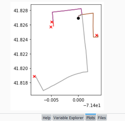
Finally, we can write the output. We convert the nested route list to a pandas dataframe and use the header row for column names, and convert that dataframe to a geodataframe, building the geometry from the WKT string, and write that out. In contrast, the origins and destinations have simple coordinates (not in WKT), and we create XY geometry from those coordinates. Writing the geodataframe out to a shapefile is straightforward, but for debugging purposes it’s helpful to see the result without having to launch GIS. We can use geopandas’s plot function to draw the resulting geometry. I’m using the Spyder IDE, which displays plots in a dedicated window (in my example the coordinate labels for the X axis look strange, as the distances I’m plotting are small).

# Create shapefiles for routes
df = pd.DataFrame(route_list, columns=header)
gdf = gpd.GeoDataFrame(df, geometry=gpd.GeoSeries.from_wkt(df["route"]),crs = 'EPSG:4326')
gdf.drop(['route'],axis=1,inplace=True) # drop the wkt text
gdf.to_file(out_file,index=True)
print('Wrote route shapefile to:',out_file,'\n')

# Create shapefiles for origins and destinations
ogdf=coords_to_gdf(origins,ogn_long,ogn_lat,out_origin)
dgdf=coords_to_gdf(dest,d_long,d_lat,out_dest)

# Plot
base=gdf.plot(column="dest_id", kind='geo',cmap="Set1")
ogdf.plot(ax=base, marker='o',color='black')
dgdf.plot(ax=base, marker='x', color='red');

In a notebook environment we can employ something like Folium more readily, which gives us a basemap and some basic interactivity for zooming around and clicking on features to see attributes. Implementing this was a more complex than I thought it would be, and took me longer to figure out compared to the routing process. I’ll return to those details in a subsequent post…

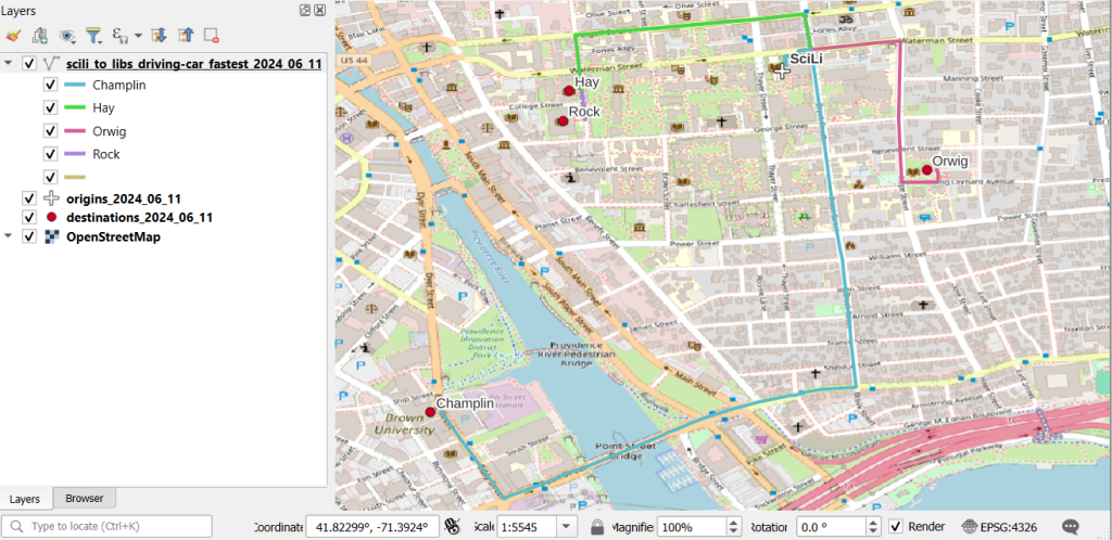
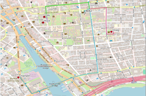
In my sample data (output rendered below in QGIS) I was plotting fastest driving distance from the Brown University Sciences Library to the other libraries in our system. Compared to Google or Apple Maps the result made sense, although the origin coordinates I used for the SciLi had an impact on the outcome (assumed you left from the loading dock behind the building as opposed to the front door as Google did, which produces different routes in this area of one-way streets). My real application was plotting distances of hundreds of miles across South America, which went well and was useful for generating different outcomes using fastest or shortest route.

Take a look at the full script in GitHub, or if programming is not your thing check out the QGIS plugin instead (activate in the Plugins menu, search for OSR). Remember to get your API key first.