census geography

The New NYC Census Factfinder

As I’m updating my presentations and handouts for the new academic year, I’m taking two new census resources for a test drive. I’ll talk about the first resource in this post.

The NYC Department of City Planning has been collating census data and publishing it for the City for quite some time. They’ve created neighborhood tabulation areas (NTAs) by aggregating census tracts, so that they could publish more reliable ACS data for small areas (since the margins of error for census tracts can be quite large) and so that New Yorkers have data for neighborhood-like areas that they would recognize. The City also publishes PUMA-level data that’s associated with the City’s Community Districts, as well as borough and city-level data. All of this information is available in a large series of Excel spreadsheets or PDFs in the form of comparison tables for each dataset.

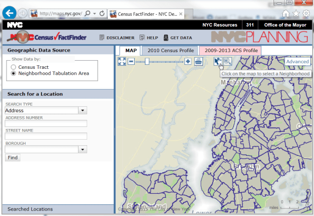
The Department of Planning also created the NYC Census Factfinder, a web-mapping interface that let’s users explore census tract and NTA level data profiles. You could plug in an address or click on the map and get a 2010 Census profile, or a demographic change profile that showed shifts between the 2000 and 2010 Census.

It was a nice application, but they’ve just made a series of updates that make it infinitely better:

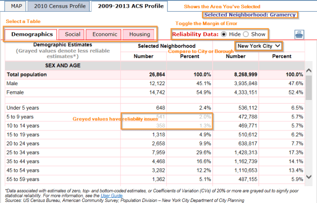
They’ve added the American Community Survey data from 2009-2013, and you can view the four demographic profile tables (demographics, social, economic, and housing) for tracts and NTAs.
Unlike many other sources, they do publish the margin of error for all of the ACS data, which is immensely important. Estimates that have a high margin of error (as defined by a coefficient of variation) appear in grey instead of solid black. While the actual margins are not shown by default, you can simply click the Show radio button to turn on the Reliability data.
Tracts or neighborhoods can be compared to the City as a whole or to an individual borough by selecting the drop down for the column header.
This is especially cool – if you’re viewing census tracts you can use the select pointer and hold down the Control key (Command key on a Mac) to select multiple tracts, and then the data tables will aggregate the tract-level data for you (so essentially you can build your own neighborhoods). What’s noteworthy here is that it also calculates the new margins of error for all of the derived estimates, AND it even calculates new medians and averages with margins of error! This is something that I’ve never seen in any other application.
In addition to searching for locations by address, you can hit the search type drop down and you have a number of additional options like Intersection, Place of Interest, and even Subway Stations.

There are a few quirks:

1. I had trouble viewing the map in Firefox – this isn’t a consistent problem but something I noticed today when I went exploring. Hopefully something temporary that will be corrected. Had no problems in IE.
2. If you want to click to select an area on the map, you have to hit the select button first (the arrow beside the zoom slider and print button) and then click on your area to select it. Just clicking on the map without hitting select first won’t do much – it will just highlight the area and tell you it’s name. Clicking the arrow button turns it blue and allows you to select features, clicking it again turns it white and lets you identify features and pan around the map.

The one bummer is that there isn’t a way to download any of the profiles – particularly the ones you custom design by selecting tracts. Hitting the Get Data button takes you out of the Factfinder and back to the page with all of the pre-compiled comparison tables. You can print the table out to a PDF for presentation purposes, but if you want a data-friendly format you’ll have to highlight and select the table on the page, copy, and paste into a spreadsheet.

These are just small quibbles that I’m sure will eventually be addressed. As is stands, with the addition of the ACS and the new features they’ve added, I’ll definitely be integrating the NYC Census Factfinder into my presentations and will be revising my NYC Neighborhood Census data handout to add it as a source. It’s unique among resources in that it provides NTA-level data in addition to tract data, has 2000 and 2010 historical change and the latest 5-year ACS (with margins of error) in one application, and allows you to build your own neighborhoods to aggregate tract data WITH new margins of error for all derived estimates. It’s well-suited for users who want basic Census demographic profiles for neighborhood-like areas in NYC.

Downloading Data for Small Census Geographies in Bulk

I needed to download block group level census data for a project I’m working on; there was one particular 2010 Census table that I needed for every block group in the US. I knew that the American Factfinder was out – you can only download block group data county by county (which would mean over 3,000 downloads if you want them all). I thought I’d share the alternatives I looked at; as I searched around the web I found many others who were looking for the same thing (i.e. data for the smallest census geographies covering a large area).

The Census FTP site at http://www2.census.gov/

This would be the first logical step, but in the end it wasn’t optimal based on my need. When you drill down through Census 2010, Summary File 1, you see a file for every state and a national file. Initially I thought – great! I’ll just grab the national file. But the national file does NOT contain the small census statistical areas – no tracts, block groups, or blocks. If you want those small areas you have to download the files for each of the states – 51 downloads. When you download the data you can also download an MS Access database, which is an empty shell with the geography and field headers, and you can import each of the text file data tables (there a lot of them for 2010 SF1) into the db and match them to the headers during import (the instructions that were included for doing this were pretty good). This is great if you need every variable in every table for every geography, but I was only interested in one table for one geography. I could just import the one text file with my table, but then I’d have to do this import process 51 times. The alternative is to use some Python to get that one text file for every state into one big file and then do the import once, but I opted for a different route.

The NHGIS at https://www.nhgis.org/

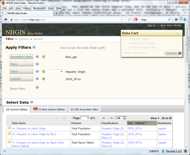
I always recommend this resource to anyone who’s looking for historical census data or boundary files, but it’s also good if you want current data for these small areas. I was able to use their query window to widdle down the selection by dataset (2010 SF1), geography (block groups), and topic (Hispanic origin and race in my case), then I was able to choose the table I needed. On the last screen before download I was able to check a box to include all 50 states plus DC and PR in one file. I had to wait a couple minutes for the request to process, then downloaded the file as a CSV and loaded it into my database. This was the best solution for my circumstances by far – one table for all block groups in the country. If you had to download a lot (or all) of the tables or variables for every block group or block it may take quite awhile, and plugging through all of those menus to select everything would be tedious – if that’s your situation it may be easier to grab everything using the Census FTP.

UExplore / Dexter at http://mcdc.missouri.edu/applications/uexplore.shtml

The Missouri Census Data Center’s UExplore / Dexter tool lets you choose a dataset and takes you to a window that resembles a file system, with a ton of files in it. The MCDC takes their extracts directly from the Census, so they’re structured in a similar way to the FTP site as state-based files. They begin with the state prefix and have a name that indicates geography – there are files for block groups, blocks, and one for everything else. There are national files (which don’t contain small census areas) that begin with ‘us’. The difference here is – when you click on a file, it launches a query window that let’s you customize the extract. The interface may look daunting at first, but it’s worth exploring (and there’s a tutorial to help guide you). You can choose from several output formats, specific variables or tables (if you don’t want them all), and there are a bunch of handy options that you can specify like aggregation or percent totals. In addition to the complete datasets, they’ve also created ‘Standard Extracts’ that have the most common variables, if you want just a core subset. While the NHGIS was the best choice for my specific need, the customization abilities in Dexter may fit your needs – and the state-level block group and block data is conveniently broken out from the other files.

Lastly…

There are a few others tools – I’ll give an honorable mention to the Summary File Retrieval tool, which is an Excel plugin that lets you tap directly into the American Community Survey from a spreadsheet. So if you wanted tracts or block groups for a wide area for but a small number of variables (I think 20 is the limit) that could be a winner, provided you’re using Excel 2007 or later and are just looking at the ACS. No dice in my case, as I needed Decennial Census data and use OpenOffice at home.

Screen Scraping Data with Python

I had a request recently for population centers (aka population centroids) for all the counties in the US. The Census provides the 2010 centroids in state level files and in one national file for download, but the 2000 centroids were provided in HTML tables on individual web pages for each state. Rather than doing the tedious work of copying and pasting 51 web pages into a spreadsheet, I figured this was my chance to learn how to do some screen scraping with Python. I’m certainly no programmer, but based on what I’ve learned (I took a three day workshop a couple years ago) and by consulting books and crawling the web for answers when I get stuck, I’ve been able to write some decent scripts for processing data.

For screen scraping there’s a must-have module called Beautiful Soup which easily let’s you parse web pages, well or ill-formed. After reading the Beautiful Soup Quickstart and some nice advice I found on a post on Stack Overflow, I was able to build a script that looped through each of the state web pages, scraped the data from the tables, and dumped it into a delimited text file. Here’s the code:

## Frank Donnelly Feb 29, 2012
## Scrapes 2000 centers of population for counties from individual state web pages
## and saves in one national-level text file.

from urllib.request import urlopen
from bs4 import BeautifulSoup

output_file=open('CenPop2000_Mean_CO.txt','a')
header=['STATEFP','COUNTYFP','COUNAME','STNAME','POPULATION','LATITUDE','LONGITUDE']
output_file.writelines(",".join(header)+"n")

url='http://www.census.gov/geo/www/cenpop/county/coucntr%s.html'

fips=['01','02','04','05','06','08','09','10',
'11','12','13','15','16','17','18','19','20',
'21','22','23','24','25','26','27','28','29','30',
'31','32','33','34','35','36','37','38','39','40',
'41','42','44','45','46','47','48','49','50',
'51','53','54','55','56']

for i in fips:
  soup = BeautifulSoup(urlopen(url %i).read())
  titleTag = soup.html.head.title
  list=titleTag.string.split()
  name=(list[4:])
  state=' '.join(name)  
 
  for row in soup('table')[1].tbody('tr'):
    tds = row('td')
    line=tds[0].string, tds[1].string, tds[2].string, state, 
    tds[3].string.replace(',',''), tds[4].string, tds[5].string

    output_file.writelines(",".join(line)+"n")     

output_file.close()

After installing the modules step 1 is to import them into the script. I initially got a little stuck here, because there are also some standard modules for working with urls (urllib and urlib2) that I’ve seen in books and other examples that weren’t working for me. I discovered that since I’m using Python 3.x and not the 2.x series, something had changed recently and I had to change how I was referencing urllib.

With that out of the way I created a a text file, a list with the column headings I want, and then wrote those column headings to my file.

Next I read in the url. Since the Census uses a static URL that varies for each state by FIPS code, I was able to assign the URL to a variable and inserted the % symbol to substitute where the FIPS code goes. I created a list of all the FIPS codes, and then I run through a loop – for every FIPS code in the list I pass that code into the url where the % place holder is, and process that page.

The first bit of info I need to grab is the name of the state, which doesn’t appear in the table. I grab the title tag from the page and save it as a list, and then grab everything from the fourth element (fifth word) to the end of the list to capture the state name, and then collapse those list elements back into one string (have to do this for states that have multiple words – New, North, South, etc.).

So we go from the HTML Title tag:

County Population Centroids for New York

To a list with elements 0 to 5:

list=[“County”, “Population”, “Centroids”, “for”, “New”, “York”]

To a shorter list with elements 4 to end:

name=[“New”,”York”]

To a string:

state=”New York”

But the primary goal here is to grab everything in the table. So we identify the table in the HTML that we want – the first table in those pages [0] is just an empty frame and the second one [1] is the one with the data. For every row (tr) in the table we can reference and grab each cell (td), and string those cells together as a line by referencing them in the list. As I string these together I also insert the state name so that it appears on every line, and for the third list element (total population in 2000) I strip out any commas (numbers in the HTML table included commas, a major no-no that leads to headaches in a csv file). After we grab that line we dump it into the output file, with each value separated by a comma and each record on it’s own line (using the new line character). Once we’ve looped through each table on each page for each state, we close the file.

There are a few variations I could have tried; I could have read the FIPS codes in from a table rather than inserting them into the script, but I preferred to keep everything together. I could have read the state names in as a list, or coupled them with the codes in a dictionary. This would have been less risky then relying on the state name in the title tag, but since the pages were well-formed and I wanted to experiment a little I went the title tag route. Instead of typing the codes in by hand I used Excel trickery to concatenate commas to the end of each code, and then concatenated all the values together in one cell so I could copy and paste the list into the script.

You can go here to see an individual state page and source, and here to see what the final output looks like. Or if you’re just looking for a national level file of 2000 population centroids for counties that you can download, look no further!

ACS Trend Reports and Census Geography Guide

I recently received my first question from someone who wanted to compare 2005-2007 ACS data with 2008-2010. With the release of the latter, we can make historical comparisons with the three year data for the first time since we have estimates that don’t overlap. We should be able to make some interesting comparisons, since the first set covers the real estate boom years (remember those?) and the second covers the Great Recession. One resource that makes such comparisons relatively painless is over at the Missouri Census Data Center. They’ve put together a really clean and simple interface called the ACS Trends Menu, which allows you to select either two one period estimates or two three period estimates and compare them for several different census geographies – states, counties, MCDs, places, metros, Congressional Districts, PUMAs, and a few others – for the entire US (not just Missouri). The end result is a profile that groups data into the Economic, Demographic, Social, and Housing categories that the Census uses for its Demographic Profile tables. The calculations for change and percent change for the estimates and margins of error are done for you.

Downloading the data is not as straightforward – the links to extract it just brought me some error messages, so it’s still a work in progress. Until then, a simple copy and paste into your spreadsheet of choice will work fine.

If you like the interface, they’ve created separate ones for downloading profiles from any of the ACS periods or from the 2010 Census. The difference here is that you’re looking at one time frame; not across time periods. The interface and the output are the same, but in these menus you can compare four different geographies at once in one profile. Unlike the Trends reports, both the ACS and 2010 Census profiles have easy, clear cut ways to download the profiles as a PDF or a spreadsheet. If you’re happy with data in a profile format and want an interface that’s a little less confusing to navigate than the American Factfinder, these are all great alternatives (and if you’re building web applications these profiles are MUCH easier to work with – you can easily build permanent links or generate them on the fly).

The US Census Bureau also recently put together a great resource called the Guide to State and Local Census Geography. They provide a census geography overview of each state: 2010 population, land area, bordering states, year of entry into the union, population centroids, and a description of how local government is organized in the state – (i.e. do they have municipal civil divisions or only incorporated cities and unincorporated land, etc). You get counts for every type of geography – how many counties, tracts, ZCTAs, and so on, AND best of all you can download all of this data directly in tab delimited files. Need a list of every county subdivision in a state, with codes, land area, and coordinates? No problem – it’s all there.

At These Coordinates

Dispatches from the Geospatial Data World