Let’s say you have different sets of points, and each set represents a distinct category of features. Maybe villages where residents speak different languages, or historical events that occurred during different epochs. Beyond plotting and symbolizing the points, perhaps you would like to create areas for each set that represent generalized territory, and you’d like to see how these areas correspond. I’ll demonstrate a few approaches for achieving this, using convex hulls, attribute table calculations, and geoprocessing tools like intersection and union. A convex hull is a minimum bounding polygon, where an area is drawn around all points in a set, where the outermost points serve as vertices for creating boundaries.
I’ll use QGIS for this example, but will mention the corresponding tools in ArcGIS Pro at the end. In QGIS we’ll use the tools that are located within the Processing Toolbox (gear icon on the toolbar). Unlike the shortcut tools under the Vector menu, these tools provide more options and allow us to process multiple files at once.
Steps in QGIS
First, we need either distinct point files for each set of features, or a single file with a categorical variable that distinctly identifies different sets of features. For this example I’ll use three distinct files that I’ve generated using phony sample data. The points are in a projected coordinate system (important!) that’s appropriate for the area I’m mapping.
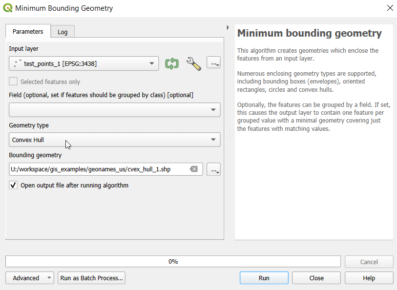
- In the QGIS Processing Toolbox, we select the Minimum Bounding Geometry (MBG) tool, and under the Geometry Type specify that we want to create a convex hull. I ran this tool for each file, creating three convex hull files (alternatively, if you had one file with distinct categories, you could use the Field option to generate separate hulls for each category). I’ve symbolized the output below, making the fill hollow and assigning an outline that matches the color of the points. This gives you a good sense for the coverage areas for the points, and how they overlap.
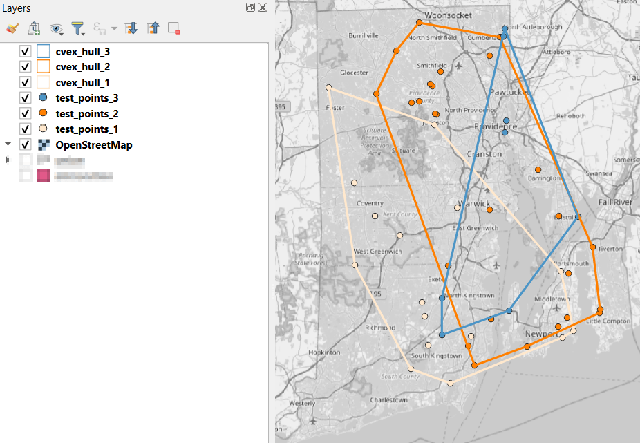
- Before running additional tools to explicitly measure overlap, we need to modify the attribute tables of the convex hulls, so we’ll have useful attributes to carry over. The MBG tool creates a new layer with an ID number, area, and perimeter. The ID is set to zero for each hull file, but we should change it to distinctly represent the file / category. With the attribute table open, we can go into an edit mode and type in a new integer value; in this case I’m assigning 1, 2, and 3 to each of the test layers. Alternatively, you could add a new field and assign it a meaningful category value.
- The units for area and perimeter match the units used by the map projection of the layer, which is why we want to use a projected coordinate system that uses meters or feet, and not a geographic one (like WGS 84 or NAD 83) that uses degrees. I’m using a state plane system, so the area is in square feet. To convert this to square miles, within the attribute table view I use the Field Calculator to add a new decimal field, and divide the value of the area by 27,878,400 (the number of sq feet in a sq mile; for metric units in meters, we’d divide by 1,000,000 to get sq km). We calculate the area directly from the polygon geometry:
area( @geometry) / 27878400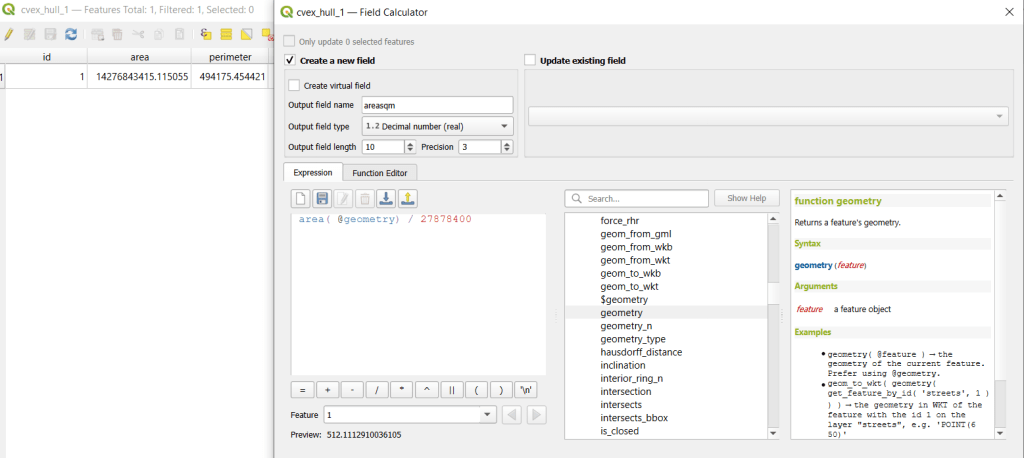
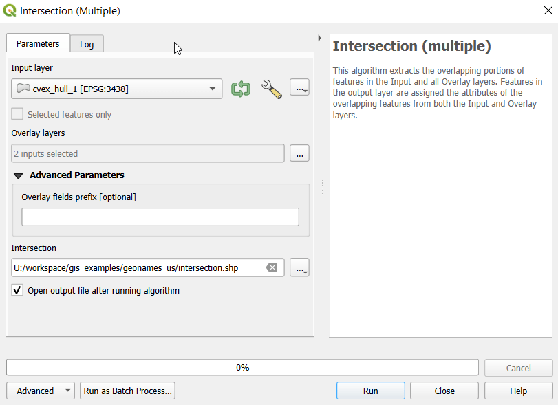
- To generate the area of intersection, we go into the Processing tool box and run the Intersection (multiple) tool. The first convex hull is the input layer, while the overlay layers are the other two hull files (in the dialog box, we check the layers we want, and then use the arrow to navigate back to the tool to run it). The output is a new file with polygon(s) that cover the area where all three layers intersect. Its attribute table contains an ID, area, and perimeter field, and we can calculate a new area field in sq miles and see how it compares to the total areas. In my example, the area where all three territories intersect covers about 112 sq miles, while the areas for the individual territories are 512, 563, and 256 sq miles respectively.

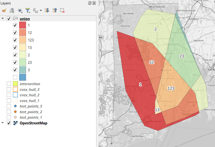
- To identify distinct areas of overlap between the territories, we return to the Processing toolbox and run the Union (multiple) tool. The dialog is similar to the intersection tool, where the first hull is the union layer and the additional hulls are overlay layers. The output of this tool is a layer with distinct polygons where the hulls coincide. The attribute table for the union layer carries over the attributes from each of the three layers, with columns suffixed with underscores and sequential integers. So if a polygon consists of area covered by hulls 1 and 2, those attributes will be filled in, while the attributes of 3 will be null. As before, we can calculate an area in sq miles for the new polygons. In this case, we’d see that the area covered by hull 1 without any overlapping hulls is 240 sq miles, the largest of all territories.

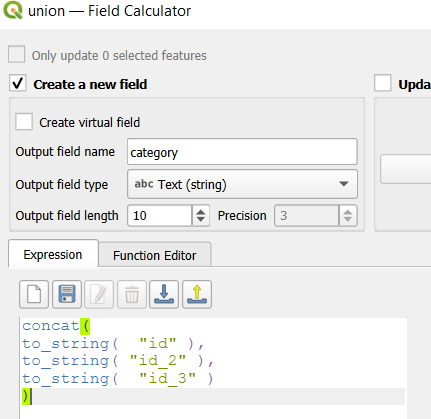
- To explicitly categorize these areas, we can add a new field in the attribute table. This will be a text field, where we take the ID numbers, convert them to strings, and concatenate them. In the example above, IDs 1 and 2 would be concatenated to 12, and since the value for 3 is null, no text is appended. (Variation – if you created distinct text-based category fields instead of using the integer IDs, you could concatenate them directly without having to convert them to strings). Using the symbology tool, we can classify the data using these new categories, and can modify the color scheme to something appropriate for displaying the contributions from each area. So a polygon with category 1 includes areas covered by the first convex hull and no others, while category 12 includes areas where hulls 1 and 2 overlapped.
concat(
to_string( "id" ),
to_string( "id_2" ),
to_string( "id_3" )
)
Additional Considerations:
- With the areas of the individual union pieces, we can compute the percentages of each territory that fall inside and outside various overlapping zones with the field calculator. For example, we can calculate the total area of the union file (which is NOT the sum of each hull, as there’s overlap between them), and then divide each feature by that total to get its percent total. The expression for doing this is below; the numerator has the name of the field that contains the area of each polygon in sq miles, while the denominator includes the calculation for the sum of all parts (alternatively you could use the QGIS Statistics tool to compute this, and hard code the total into the formula):
area_part / (sum(area( geometry(@feature)))/27878400) *100- If the idea is to create areas of territory that the points exert influence on, you may want to add a buffer to each hull, to account for the fact that the outer points that form the boundaries will exert influence on both sides of the boundary. Use the Processing – Buffer tool. For the buffer distance, you can use an arbitrary value that makes sense for the circumstances. Or you can generate a relative value that represents a fraction of each convex hull’s area. The output of the buffer tool would then serve as the input to the intersection and union tools.
- These examples focus on area. If the number of points that falls within the areas is important, you can use the Points in Polygon tool on each of the hulls to count points, and then do the same for the output of the intersection and union tools to get the different points counts for each set of polygons.
ArcGIS Pro Corollaries
Following the same steps above for QGIS, but with ArcGIS Pro:
- In the red toolbox, the Minimum Boundary Geometry tool is used to create convex halls. It’s quite similar to the one in QGIS: specify the geometry type, and there is an option to Group (if you have one file with categories). If you leave the Add geometry characteristics box unchecked, it will still compute basic area and perimeter; the checkbox adds a bunch of additional fields.
- Unlike QGIS, ArcGIS will not allow you to modify its OBJECTID field. To create a unique value for each hull, you will have to open the attribute table and use the Calculate tool to create a category field (integer or text). To ensure that you can carry it over, in ArcGIS you need to give this column a different name in each hull: cat1, cat2, cat3. Set the value at the bottom in the expression box.
- You can use the calculate tool in the attribute table to generate an area column in sqft or sqkm, or use the Calculate Geometry Tool in the toolbox instead. The latter is actually simpler: create a new column, and choose Area and the output units.
- The Intersect tool will create the intersection, and functions similarly to QGIS.
- The Union tool creates the union, and also functions similarly.
- Creating the category field in the union file is a bit more complicated, as ArcGIS assigns values of 0 instead of NULL for non-overlapping polygons. In the Calculate window, with the input file as Union
and the field as category, change the Expression type to Arcade (ESRI’s scripting language). First, run an expression to concatenate the categories and convert integers to strings (if necessary). Then, replace that expression with a second one that replace the zeros with nothing.
Concatenate(TEXT($feature.cat1)+
TEXT($feature.cat2)+
TEXT($feature.cat3)
)
Replace($feature.category,'0','')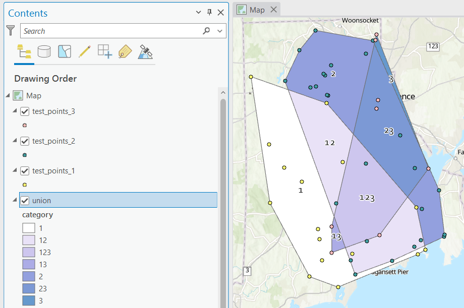
Conclusion
This is a basic approach, appropriate for certain use cases where you want to generate areas from points; particularly when different point sets have a well defined category, so there’s no question of how to group them. Also appropriate where you don’t have – or don’t want – hard boundaries between sets of points and want to see areas of overlap. More sophisticated methods exist for separating points into clusters based on density, distance, and similar attributes, such as K-Means and DB Scan. You can generate non-overlapping territories for individual points using Thiessen / Voronoi polygons, and for points with a sufficiently high density, you can generate rasters with kernel tools.

You must be logged in to post a comment.